Capacity Estimation for System Design: Traffic, Storage, Bandwidth, and Headroom
Published:
1. Introduction
What Capacity Estimation Is For
A system-design estimate converts a product workload into an infrastructure model:
users and behavior
  -> operations per day
  -> peak operations per second
  -> concurrent work
  -> network, storage, memory, and compute demand
  -> capacity with failure headroom
The result is not a purchasing order. Early estimates are built from uncertain inputs and simplified relationships. Their purpose is to determine the architecture’s shape and locate the dimensions that deserve measurement.
For example, an estimate may reveal that:
- request throughput is small but response bandwidth is dominant;
- average traffic is easy but a regional failover is not;
- application servers are inexpensive but the durable working set is large;
- client requests are modest but fanout creates heavy database traffic;
- storage capacity fits comfortably while write IOPS do not;
- connection count, rather than requests per second, limits the service.
The useful output is therefore not one impressive number. It is a model that connects assumptions to consequences.
Estimation Is Not Benchmarking
Arithmetic cannot determine how many requests a particular server process can handle. That depends on implementation, hardware, query plans, payloads, dependencies, latency targets, and the point at which the system is considered saturated.
Capacity estimation can tell us:
the service needs approximately 10,000 peak requests per second
A benchmark or production measurement must tell us:
one instance sustains 1,200 representative requests per second
at the target latency and utilization
Only then can the model translate demand into an instance count.
Prefer Ranges to False Precision
Inputs such as daily active users, peak multiplier, cache hit ratio, and record size are rarely exact. A result such as:
9,742.38 requests per second
does not become accurate merely because it has decimal places. A more honest statement is:
base estimate: 10,000 peak requests per second
plausible range: 6,000 to 18,000
The range exposes uncertainty and encourages sensitivity analysis.
2. Units and Conversion Rules
Decimal and Binary Prefixes
Capacity discussions often mix decimal storage units with binary memory units. State the convention before calculating.
| Name | Decimal value | Binary name | Binary value |
|---|---|---|---|
| kilobyte, KB | 1,000 bytes | kibibyte, KiB | 1,024 bytes |
| megabyte, MB | 1,000,000 bytes | mebibyte, MiB | 1,048,576 bytes |
| gigabyte, GB | 1,000,000,000 bytes | gibibyte, GiB | 1,073,741,824 bytes |
| terabyte, TB | 1,000,000,000,000 bytes | tebibyte, TiB | 1,099,511,627,776 bytes |
Network rates and storage-device specifications are commonly decimal. Memory allocations and operating-system output often use powers of two, sometimes while displaying the labels KB or GB. Either convention is usable if it is applied consistently.
This article uses decimal units for traffic and persistent storage unless a binary unit is written explicitly.
Bits and Bytes
Network interfaces are frequently described in bits per second:
1 byte = 8 bits
1 GB/s = 8 Gb/s
Do not compare an estimate in gigabytes per second directly with a network interface rated in gigabits per second.
Time Conversions
1 minute = 60 seconds
1 hour   = 3,600 seconds
1 day    = 86,400 seconds
For mental arithmetic:
1 day is approximately 100,000 seconds
The approximation is useful for an interview whiteboard, but a reproducible calculator should use 86,400.
Useful daily-rate conversions are:
| Operations per day | Average operations per second |
|---|---|
| 1 million | 11.6 |
| 10 million | 115.7 |
| 100 million | 1,157 |
| 1 billion | 11,574 |
Keep Units in the Formula
Dimensional analysis catches mistakes:
requests        bytes
--------   *   -------   = bytes/second
 second        request
Likewise:
records      bytes       days
-------  *  -------  *  ----  = bytes
 day        record       retention period
If the units do not cancel to the quantity being estimated, the formula is wrong even if the arithmetic is correct.
3. Build the Workload Model
Start With Behavior
Do not begin by guessing server count. Begin with actions:
population
  -> active population
  -> sessions per active user
  -> actions per session
  -> operations generated by each action
For a read-heavy media metadata service:
5 million daily active users
20 reads per active user per day
2 writes per active user per day
The logical daily operations are:
reads/day  = 5,000,000 * 20 = 100,000,000
writes/day = 5,000,000 *  2 =  10,000,000
total/day  = 110,000,000
Separate Workload Classes
An average across unrelated operations hides resource differences. Model at least the dominant paths separately:
| Operation | Frequency | Request size | Response size | Expected cost |
|---|---|---|---|---|
| Read metadata | High | Small | Medium | Cacheable read |
| Create record | Medium | Medium | Small | Durable write |
| Search | Medium | Small | Large | CPU and index intensive |
| Upload object | Low | Very large | Small | Bandwidth and storage intensive |
A system serving 10,000 metadata reads per second is not equivalent to one serving 10,000 uploads per second.
Distinguish Product Events From Internal Operations
One user action may fan out:
create post
  -> authenticate
  -> write primary record
  -> update two indexes
  -> append event
  -> invalidate cache
  -> notify followers
If one external write causes four durable writes, the storage system sees four write operations per user action before replication or compaction is counted.
Use explicit fanout factors:
internal_write_rate =
    external_write_rate * writes_per_action
Record Every Assumption
A useful estimate starts with a table that another engineer can challenge:
| Assumption | Base value | Why it matters |
|---|---|---|
| Daily active users | 5 million | Scales daily operation count |
| Reads per user per day | 20 | Drives read throughput and egress |
| Writes per user per day | 2 | Drives durable growth |
| Peak multiplier | 8x | Converts average to peak provisioning |
| Average request payload | 500 bytes | Drives ingress |
| Average response payload | 1,500 bytes | Drives egress |
| Durable record size | 1,000 bytes | Drives logical storage |
| Retention | 365 days | Drives retained dataset |
| Cache hit ratio | 90% | Determines origin-read load |
| p95 service time | 120 ms | Approximates peak concurrency |
Assumptions are not weaknesses in the model. Hidden assumptions are.
4. From Daily Volume to Request Rate
Average Rate
For an operation count N_day:
average rate = N_day / 86,400
For 100 million reads per day:
100,000,000 / 86,400
    = 1,157 average reads/second
For 10 million writes per day:
10,000,000 / 86,400
    = 116 average writes/second
The total average rate is approximately:
1,157 + 116 = 1,273 requests/second
Average Is Not Provisioning Load
Traffic is shaped by time zones, work schedules, live events, retries, batch jobs, marketing campaigns, and client synchronization. Capacity must normally be based on a measured or assumed peak.
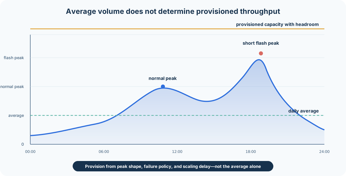
With an 8x peak multiplier:
peak reads  = 1,157 * 8 = 9,259 reads/second
peak writes =   116 * 8 =   926 writes/second
peak total  = 1,273 * 8 = 10,185 requests/second
The peak multiplier should come from observed traffic where possible. If it is unknown, calculate low, base, and high cases rather than silently assuming one.
Different Peaks Can Occur at Different Times
Read, write, batch, and regional-failover peaks may not coincide:
morning: notification reads
evening: content creation
midnight: compaction and analytics export
incident: retries and regional failover
Blindly adding every independent maximum can overestimate capacity. Assuming they never overlap can underestimate it. Model the combinations that can plausibly occur together.
Arrival Distribution Matters
Ten thousand requests uniformly spread across one second are easier to absorb than ten thousand arriving in the same few milliseconds. Per-second averages hide microbursts.
Buffers can smooth short bursts, but only by trading resource use for queueing latency. Latency-sensitive synchronous traffic needs both a throughput estimate and a burst model.
5. Concurrency and Little’s Law
Rate Is Not Concurrency
Requests per second measures arrival rate. Concurrent requests measure how much work is in flight.
Little’s Law relates average in-flight work L, arrival rate lambda, and average time in the system W:
L = lambda * W
If the peak arrival rate is 10,185 requests per second and average time in the system is 120 milliseconds:
L = 10,185 requests/second * 0.120 seconds
  = 1,222 concurrent requests
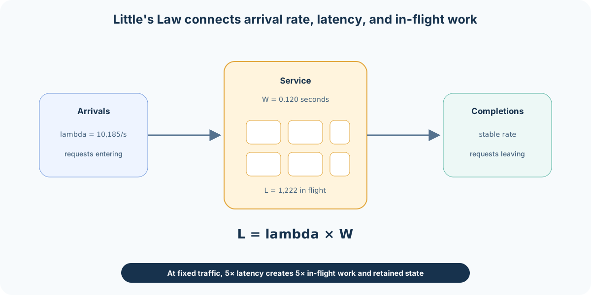
If latency increases to 600 milliseconds without a traffic increase:
L = 10,185 * 0.600
  = 6,111 concurrent requests
This is why a dependency slowdown creates memory, socket, thread, and connection-pool pressure before request rate changes.
Use the Correct Time
For average concurrency, use average time. For a conservative queue, connection-pool, or memory estimate, a high-percentile duration may be useful, but it no longer produces the mathematical average promised by Little’s Law. State the interpretation:
average concurrency model: average rate * average duration
stress approximation: peak rate * p95 or deadline duration
Long-Lived Connections Need a Separate Model
WebSockets, database sessions, and streaming RPCs are not well represented by ordinary request concurrency:
open connections =
    concurrently connected users * connections per user
Then estimate:
connection memory =
    open connections * bytes of state per connection
A million idle connections may generate few requests per second while still consuming file descriptors, kernel socket buffers, userspace state, and heartbeat traffic.
6. Network Bandwidth
Calculate Ingress and Egress Separately
For peak request rate (R):
ingress bytes/second =
    R * average request bytes

egress bytes/second =
    R * average response bytes
At 10,185 peak requests per second:
ingress = 10,185 * 500 bytes
        = 5.09 MB/s
        = 40.7 Mb/s

egress  = 10,185 * 1,500 bytes
        = 15.28 MB/s
        = 122.2 Mb/s
These figures describe application payloads. Actual wire traffic also includes protocol framing, TLS, retransmissions, acknowledgements, and sometimes encapsulation. Measure the ratio under representative traffic rather than adding an arbitrary universal percentage.
Account for Internal Hops
One external response may cross several internal network boundaries:
storage -> service
service -> proxy
proxy -> client
If the service calls three dependencies and sends an event, external bandwidth alone underestimates east-west traffic.
For a fanout operation:
internal bandwidth =
    request rate
    * calls per request
    * average internal payload
Convert Rate Into Daily Transfer
At an average response rate of 1,273 responses per second and 1,500 bytes per response:
daily response payload =
    1,273 * 1,500 * 86,400
    = 165 GB/day
Daily and monthly transfer matter for cost even when the network interface has ample throughput.
Compression Changes CPU as Well as Bandwidth
Compression may reduce network bytes while increasing CPU time and latency. The right model includes both:
compressed egress = raw egress * compression ratio
additional CPU    = measured compression CPU per byte
Do not assume that smaller payloads are free.
7. Persistent Storage
Begin With Logical Data
For fixed-size records:
logical storage =
    records per day
    * bytes per record
    * retention days
For 10 million new 1 KB records per day retained for 365 days:
logical storage =
    10,000,000 * 1,000 * 365
    = 3.65 TB
This is only the application payload.
Estimate the Record, Not Just the Obvious Field
A durable record may contain:
identifier
owner identifier
timestamps
status and flags
payload
encoding overhead
row or object metadata
Indexes add separate entries. Variable-length formats add keys, offsets, type markers, and allocation overhead. Small records often have a larger percentage of metadata overhead than large objects.
A useful record-size estimate is:
| Component | Example bytes |
|---|---|
| Identifiers | 32 |
| Timestamps and flags | 24 |
| Payload | 800 |
| Encoding and row overhead | 144 |
| Total | 1,000 |
Verify the estimate later with serialized production-shaped data.
From Logical to Physical Storage
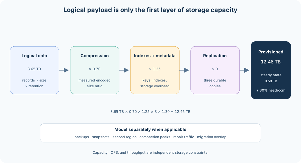
Physical storage may include compression, indexes, replication, temporary compaction space, snapshots, and operational headroom:
physical steady state =
    logical data
    * compression ratio
    * index and metadata factor
    * replica factor
Using:
logical data             = 3.65 TB
compression ratio        = 0.70
index and metadata factor = 1.25
replica factor           = 3
gives:
3.65 * 0.70 * 1.25 * 3
    = 9.58 TB
With 30 percent operational headroom:
9.58125 * 1.30 = 12.46 TB provisioned
Storage Capacity Is Not Storage Throughput
A dataset can fit on a disk while exceeding its sustainable IOPS or bandwidth. Estimate separately:
read IOPS
write IOPS
sequential throughput
random throughput
write amplification
background maintenance traffic
An LSM-based database may turn one logical write into write-ahead-log traffic, memtable flushes, and repeated compaction writes. A replicated database also writes multiple copies.
Retention Is a Lifecycle
Not every byte needs the same storage tier:
0-7 days    -> hot indexed storage
8-90 days   -> warm queryable storage
91-365 days -> cold object storage
beyond      -> delete or archive
Tiering changes cost and latency but also adds migration, restoration, and deletion workflows.
8. Compute Capacity
Use Measured Service Capacity
Suppose a representative load test shows one application instance can sustain:
1,200 requests/second
at <= 60% CPU
while meeting the p99 latency target
For 10,185 peak requests per second:
instances for normal peak =
    ceil(10,185 / 1,200)
    = 9
The phrase “representative load test” matters. The test should include the actual read/write mix, payload distribution, dependency latency, connection reuse, TLS behavior, and logging.
A CPU-Time Cross-Check
If a request consumes 2.5 milliseconds of CPU on average:
CPU cores fully busy =
    requests/second * CPU seconds/request

    = 10,185 * 0.0025
    = 25.5 cores
At a target CPU utilization of 60 percent:
provisioned cores =
    25.5 / 0.60
    = 42.5 cores
This is a cross-check, not a replacement for a benchmark. Lock contention, memory bandwidth, garbage collection, I/O waits, and tail latency can limit the service before average CPU reaches the target.
Include Background Work
Application traffic may share compute with:
- health checks;
- metrics and tracing;
- cache refresh;
- asynchronous callbacks;
- certificate rotation;
- garbage collection;
- log serialization;
- deployment overlap.
If these costs are excluded from the benchmark, add them explicitly or lower the target utilization.
9. Memory and Cache Capacity
Estimate the Working Set
A cache does not necessarily need to hold the entire durable dataset. It needs enough space for the useful working set:
cache bytes =
    hot items
    * physical bytes per cached item
    * cache replica factor
Physical bytes per item include more than the serialized value:
key
value
allocator overhead
hash-table or index entry
expiration metadata
fragmentation
If 50 million hot items consume an estimated 1,200 bytes each:
one cache copy =
    50,000,000 * 1,200
    = 60 GB
With two copies and 20 percent headroom:
60 GB * 2 * 1.20 = 144 GB
Hit Ratio Determines Origin Load
For a 90 percent cache hit ratio:
origin read rate =
    total read rate * (1 - hit ratio)
At 9,259 peak reads per second:
origin reads =
    9,259 * 0.10
    = 926 reads/second
If the hit ratio falls to 70 percent:
origin reads =
    9,259 * 0.30
    = 2,778 reads/second
A 20 percentage-point hit-ratio reduction triples origin load. Database capacity should therefore be tested against cold-cache startup, mass expiration, and cache failure rather than only steady-state hits.
Cache Hit Ratio Is Workload Dependent
Cache capacity and hit ratio are not connected by one universal linear formula. The result depends on popularity distribution, object size, expiration, eviction policy, and request correlation.
Estimate the working set to choose an initial scale, then validate it with a trace or production metrics.
Memory for In-Flight Work
Request handling also consumes memory:
in-flight memory =
    concurrent requests * bytes per request state
If 1,222 concurrent requests each retain 64 KB across request buffers, parsed state, and dependency responses:
1,222 * 64 KB = 78.2 MB
The mean is rarely the dangerous case. Large uploads, slow clients, retries, and downstream stalls can retain more bytes for longer. Use per-request and global buffer limits.
10. Database and Dependency Load
Translate Requests Into Database Operations
Application RPS is not database RPS. For each request class, enumerate the calls it creates:
| Request | Rate | Cache misses | Database reads | Database writes |
|---|---|---|---|---|
| Read metadata | 9,259/s | 10% | 926/s | 0 |
| Create record | 926/s | N/A | 0 | 926/s |
| Update indexes | Generated by writes | N/A | 0 | 1,852/s |
If every logical write updates two secondary indexes:
logical database writes =
    926 primary writes
    + 1,852 index writes
    = 2,778 writes/second
Replication and storage-engine write amplification occur below this count.
Fanout Multiplies Dependency Load
If every external request makes three synchronous RPCs:
dependency calls =
    external request rate * 3
At 10,185 peak requests per second, that is 30,555 dependency calls per second. The dependencies may become the capacity constraint before the frontend service.
Connection Pools Need a Queueing Model
A database pool must support useful concurrency, not the full arrival rate:
database concurrency =
    database operation rate * operation latency
For 2,778 operations per second at 15 milliseconds average latency:
2,778 * 0.015 = 41.7 concurrent operations
A pool somewhat larger than this may absorb variation. A pool many times larger may simply allow more work to queue inside the database. Pool sizing should be tested against database saturation and request deadlines.
Count Background and Repair Traffic
Database capacity must leave room for:
- replication;
- compaction;
- backups;
- consistency checks;
- read repair;
- anti-entropy;
- index construction;
- schema migration;
- rebalancing after a node failure.
Steady-state foreground traffic is only part of the workload.
11. Reliability and Failure Headroom
Normal-Peak Capacity Is Not Enough
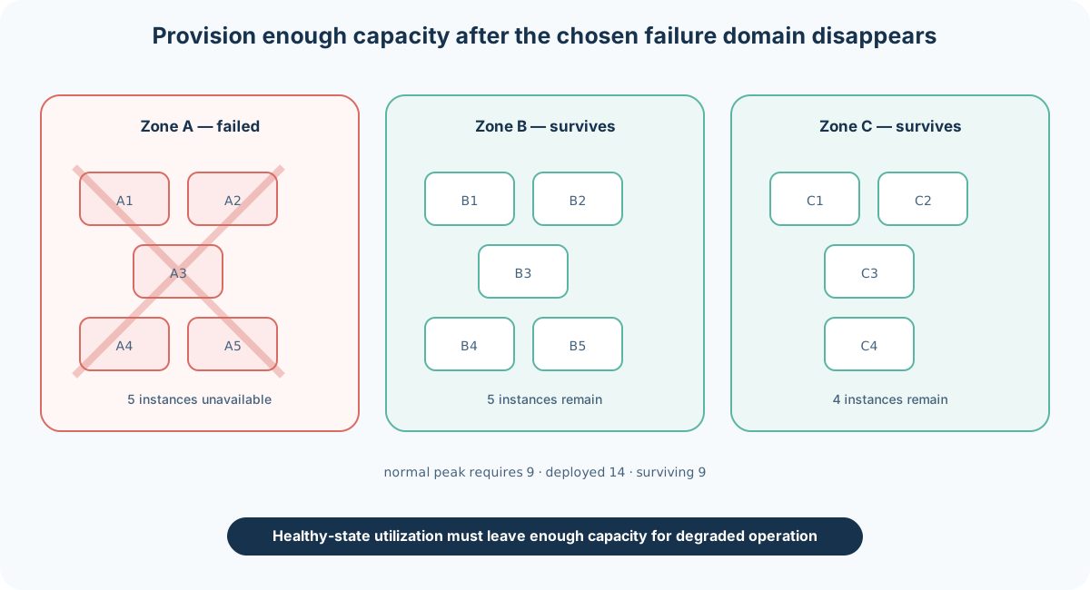
Nine instances may serve the normal peak, but nine is not necessarily the deployment target. The fleet must survive maintenance and expected failures.
If instances are spread evenly across three availability zones, losing one zone removes approximately one third of the fleet. To preserve peak capacity:
zone-safe instances =
    ceil(normal_peak_instances / remaining_fraction)

    = ceil(9 / (2/3))
    = 14
With 14 instances distributed as 5, 5, and 4, losing a five-instance zone leaves nine instances.
Headroom Has Several Purposes
Capacity margins cover different risks:
- traffic forecast error;
- an availability-zone or node failure;
- rolling deployment overlap;
- autoscaling delay;
- cold caches;
- dependency slowdown;
- retry traffic;
- unexpected record or payload growth.
Do not combine them into one unexplained percentage. A failure-domain calculation and a forecast uncertainty range answer different questions.
Target Utilization Is a Latency Decision
Running at 100 percent theoretical throughput leaves no room for bursts or failure. Queueing delay also rises sharply as a constrained resource approaches saturation.
The target may be:
CPU <= 60%
database connections <= 70%
network <= 50% of tested sustainable rate
storage <= 70% full
These are examples, not universal constants. The correct targets come from the system’s latency curve, scaling speed, recovery behavior, and failure policy.
Autoscaling Does Not Remove Base Capacity
Autoscaling reacts after a signal crosses a threshold. New capacity needs time to provision, initialize, warm caches, load configuration, and pass health checks.
The service needs enough pre-existing capacity to survive:
detection time
+ provisioning time
+ warm-up time
Fast unpredictable bursts require scheduled scaling, queueing, load shedding, or more standing headroom.
12. A Complete Worked Example
Product Assumptions
Consider the read-heavy media metadata service introduced earlier:
| Input | Value |
|---|---|
| Daily active users | 5,000,000 |
| Reads per user per day | 20 |
| Writes per user per day | 2 |
| Peak multiplier | 8x |
| Average request | 500 bytes |
| Average response | 1,500 bytes |
| Durable record | 1,000 bytes |
| Retention | 365 days |
| Compression ratio | 0.70 |
| Index and metadata factor | 1.25 |
| Storage replica factor | 3 |
| Storage headroom | 30% |
| Cache hit ratio | 90% |
| Hot cache items | 50,000,000 |
| Physical cached item | 1,200 bytes |
| Cache replicas | 2 |
| Cache headroom | 20% |
| Peak service time approximation | 120 ms |
| Tested instance capacity | 1,200 RPS |
| Availability zones | 3 |
Traffic
daily reads  = 5,000,000 * 20 = 100,000,000
daily writes = 5,000,000 *  2 =  10,000,000

average reads  = 100,000,000 / 86,400 = 1,157/s
average writes =  10,000,000 / 86,400 =   116/s

peak reads  = 1,157 * 8 = 9,259/s
peak writes =   116 * 8 =   926/s
peak total  = 10,185/s
Concurrency
stress concurrency approximation =
    10,185 * 0.120
    = 1,222 in-flight requests
Network
peak ingress =
    10,185 * 500
    = 5.09 MB/s
    = 40.7 Mb/s

peak egress =
    10,185 * 1,500
    = 15.28 MB/s
    = 122.2 Mb/s

average daily response payload =
    1,273 * 1,500 * 86,400
    = 165 GB/day
Storage
logical retained data =
    10,000,000 * 1,000 * 365
    = 3.65 TB

physical steady state =
    3.65 * 0.70 * 1.25 * 3
    = 9.58 TB

provisioned with 30% headroom =
    9.58125 * 1.30
    = 12.46 TB
This estimate does not yet include backups, temporary compaction peaks, or a second region. Those must be added if the proposed architecture uses them.
Cache
peak origin reads =
    9,259 * (1 - 0.90)
    = 926 reads/second

cache memory =
    50,000,000 * 1,200 * 2 * 1.20
    = 144 GB
Application Fleet
normal-peak instances =
    ceil(10,185 / 1,200)
    = 9

instances surviving one of three zones =
    ceil(9 / (2/3))
    = 14
The result is a starting architecture:
14 application instances across 3 zones
cache tier sized for approximately 144 GB
database sustaining at least 926 origin reads/s
and 926 primary writes/s before index and engine amplification
approximately 12.46 TB provisioned primary storage
plus separately modelled backups and cross-region copies
The next step is not to accept these numbers. It is to test the most sensitive assumptions.
13. A Reproducible Calculator
Keep Inputs Separate From Derived Values
The following Python program implements the worked example. It is deliberately small enough to audit and modify:
from dataclasses import dataclass
from math import ceil

SECONDS_PER_DAY = 86_400
BITS_PER_BYTE = 8


@dataclass(frozen=True)
class CapacityInputs:
    daily_active_users: int
    reads_per_user_day: float
    writes_per_user_day: float
    peak_multiplier: float

    request_bytes: int
    response_bytes: int
    service_time_ms: float

    record_bytes: int
    retention_days: int
    compression_ratio: float
    index_metadata_factor: float
    storage_replicas: int
    storage_headroom: float

    cache_hit_ratio: float
    hot_cache_items: int
    cached_item_bytes: int
    cache_replicas: int
    cache_headroom: float

    tested_rps_per_instance: float
    availability_zones: int


def estimate(model: CapacityInputs) -> dict[str, float | int]:
    daily_reads = (
        model.daily_active_users * model.reads_per_user_day
    )
    daily_writes = (
        model.daily_active_users * model.writes_per_user_day
    )

    average_reads = daily_reads / SECONDS_PER_DAY
    average_writes = daily_writes / SECONDS_PER_DAY
    average_total = average_reads + average_writes

    peak_reads = average_reads * model.peak_multiplier
    peak_writes = average_writes * model.peak_multiplier
    peak_total = peak_reads + peak_writes

    peak_concurrency = (
        peak_total * model.service_time_ms / 1_000
    )

    ingress_bytes_second = peak_total * model.request_bytes
    egress_bytes_second = peak_total * model.response_bytes
    daily_egress_bytes = (
        average_total
        * model.response_bytes
        * SECONDS_PER_DAY
    )

    logical_storage_bytes = (
        daily_writes
        * model.record_bytes
        * model.retention_days
    )
    physical_storage_bytes = (
        logical_storage_bytes
        * model.compression_ratio
        * model.index_metadata_factor
        * model.storage_replicas
    )
    provisioned_storage_bytes = (
        physical_storage_bytes
        * (1 + model.storage_headroom)
    )

    origin_peak_reads = (
        peak_reads * (1 - model.cache_hit_ratio)
    )
    cache_bytes = (
        model.hot_cache_items
        * model.cached_item_bytes
        * model.cache_replicas
        * (1 + model.cache_headroom)
    )

    normal_instances = ceil(
        peak_total / model.tested_rps_per_instance
    )
    surviving_fraction = (
        model.availability_zones - 1
    ) / model.availability_zones
    zone_safe_instances = ceil(
        normal_instances / surviving_fraction
    )

    return {
        "average_rps": average_total,
        "peak_read_rps": peak_reads,
        "peak_write_rps": peak_writes,
        "peak_total_rps": peak_total,
        "peak_concurrency": peak_concurrency,
        "ingress_mb_s": ingress_bytes_second / 1e6,
        "ingress_mbit_s": (
            ingress_bytes_second * BITS_PER_BYTE / 1e6
        ),
        "egress_mb_s": egress_bytes_second / 1e6,
        "egress_mbit_s": (
            egress_bytes_second * BITS_PER_BYTE / 1e6
        ),
        "daily_egress_gb": daily_egress_bytes / 1e9,
        "logical_storage_tb": logical_storage_bytes / 1e12,
        "provisioned_storage_tb": (
            provisioned_storage_bytes / 1e12
        ),
        "origin_peak_read_rps": origin_peak_reads,
        "cache_gb": cache_bytes / 1e9,
        "normal_instances": normal_instances,
        "zone_safe_instances": zone_safe_instances,
    }


inputs = CapacityInputs(
    daily_active_users=5_000_000,
    reads_per_user_day=20,
    writes_per_user_day=2,
    peak_multiplier=8,
    request_bytes=500,
    response_bytes=1_500,
    service_time_ms=120,
    record_bytes=1_000,
    retention_days=365,
    compression_ratio=0.70,
    index_metadata_factor=1.25,
    storage_replicas=3,
    storage_headroom=0.30,
    cache_hit_ratio=0.90,
    hot_cache_items=50_000_000,
    cached_item_bytes=1_200,
    cache_replicas=2,
    cache_headroom=0.20,
    tested_rps_per_instance=1_200,
    availability_zones=3,
)

for name, value in estimate(inputs).items():
    if isinstance(value, float):
        print(f"{name:28s} {value:,.2f}")
    else:
        print(f"{name:28s} {value:,}")
The expected output is:
average_rps                  1,273.15
peak_read_rps                9,259.26
peak_write_rps                 925.93
peak_total_rps              10,185.19
peak_concurrency             1,222.22
ingress_mb_s                     5.09
ingress_mbit_s                  40.74
egress_mb_s                     15.28
egress_mbit_s                  122.22
daily_egress_gb                165.00
logical_storage_tb               3.65
provisioned_storage_tb           12.46
origin_peak_read_rps            925.93
cache_gb                        144.00
normal_instances                     9
zone_safe_instances                 14
The calculator does not make the assumptions correct. It makes them visible, repeatable, and easy to vary.
14. Sensitivity and Uncertainty
Vary the Inputs That Drive Architecture
Not every assumption deserves equal attention. Test the ones that change the architecture or dominate cost:
| Variable | Low | Base | High |
|---|---|---|---|
| Daily active users | 3 million | 5 million | 8 million |
| Peak multiplier | 5x | 8x | 12x |
| Response payload | 1 KB | 1.5 KB | 4 KB |
| Cache hit ratio | 95% | 90% | 70% |
| Retention | 90 days | 365 days | 730 days |
| Tested instance capacity | 1,500 RPS | 1,200 RPS | 800 RPS |
The high case is not created by multiplying every pessimistic input together unless they can plausibly coincide. Construct scenarios:
growth scenario:
  more users and normal payloads

incident scenario:
  normal users, lower cache hit ratio, retries

launch scenario:
  higher peak multiplier and cold application fleet

retention scenario:
  normal traffic and longer data lifetime
Find Breakpoints
A useful estimate identifies thresholds:
At what DAU does one database shard exceed write capacity?
At what response size does egress saturate the regional link?
At what hit ratio does the origin database overload?
How many instances are required after one zone fails?
When does the hot working set stop fitting in memory?
Breakpoints guide monitoring and scaling plans more effectively than one base number.
Reconcile the Model With Reality
After launch, compare:
estimated RPS              vs observed RPS
estimated peak multiplier  vs observed traffic curve
estimated record size      vs serialized and indexed size
estimated cache item size  vs allocator memory
tested instance capacity   vs production latency curve
estimated fanout           vs traced dependency calls
Update the model. A capacity estimate should become a living operational tool, not remain an interview artifact.
15. Common Estimation Errors
Treating Daily Volume as Peak Throughput
Dividing by 86,400 produces an average. Provisioning directly from that number assumes perfectly uniform traffic.
Mixing Bits and Bytes
A 1 Gb/s interface does not carry 1 GB/s. Before protocol overhead, the theoretical conversion is 125 MB/s.
Multiplying User Count Directly by RPS
Registered users are not simultaneously active users. Daily active users are not concurrent users. Concurrent users do not necessarily send one request every second.
Build the behavioral chain explicitly.
Using Payload Size as Physical Record Size
Serialization, keys, indexes, metadata, replication, snapshots, and temporary maintenance space all add bytes.
Ignoring Read and Write Amplification
One application operation may become multiple database, index, log, and replica operations.
Deriving Server Count Without Measurement
Statements such as “one server handles 10,000 RPS” are meaningless without a workload, hardware profile, latency target, and saturation definition.
Applying Headroom Twice Without Saying So
If benchmark capacity already uses a 60 percent CPU target, then adding another 40 percent “CPU headroom” may count the same margin twice. Failure headroom, forecast uncertainty, and utilization targets should be named separately.
Ignoring the Failure Case
A fleet that meets peak demand only when every node and availability zone is healthy is not highly available.
Presenting Precision Without Uncertainty
Round numbers appropriately and show which input controls the result.
16. A Practical Estimation Workflow
Step 1: Define Scope
Write down:
- geography and regions;
- user population;
- included product operations;
- latency target;
- retention;
- expected failure domain;
- whether the estimate covers steady state, peak, or disaster recovery.
Step 2: Model Product Behavior
For each important action, estimate:
active users
* actions per active user
* internal operations per action
Separate reads, writes, uploads, searches, background jobs, and long-lived connections.
Step 3: Calculate Average and Peak Rates
average rate = operations/day / 86,400
peak rate    = average rate * measured or assumed peak factor
Use different peak factors where workloads have different shapes.
Step 4: Derive Resource Demand
Calculate:
- concurrency;
- ingress and egress;
- durable logical and physical storage;
- working-set memory;
- database and dependency operations;
- connection and buffer state;
- benchmark-based compute.
Step 5: Apply Reliability Requirements
Test the model after:
- one instance fails;
- one availability zone fails;
- a cache becomes cold;
- a dependency slows;
- a regional failover adds traffic;
- a rolling deployment temporarily duplicates capacity.
Step 6: Run Sensitivity Cases
Vary the two or three assumptions most likely to change the architecture.
Step 7: State the Result as a Range
A concise conclusion might be:
The base workload is approximately 10,000 peak RPS,
with a plausible 6,000-18,000 RPS range.

Fourteen measured application instances preserve base peak
after one of three zones fails.

Primary data needs approximately 12.5 TB after compression,
indexes, three replicas, and free-space headroom, excluding
backups and a second region.

The database is most sensitive to cache hit ratio:
origin reads rise from about 463/s at 95% hits
to about 2,778/s at 70% hits.
That statement is more useful than a large table with unexplained precision.
17. Conclusion
Capacity estimation is a chain of explicit relationships:
user behavior
-> daily operations
-> average and peak rates
-> concurrency and fanout
-> bandwidth, storage, memory, database, and compute demand
-> failure-safe provisioned capacity
The strongest estimates keep units visible, separate workload classes, model average and peak independently, and distinguish logical data from physical storage. They use Little’s Law to connect latency with concurrency, translate cache hit ratio into origin load, and derive instance count from representative measurements rather than folklore.
The final numbers should remain approximate. The rigor comes from making each assumption challengeable, each formula reproducible, and each failure case explicit. An estimate becomes operationally valuable when it is later compared with measurements and updated as the workload changes.
Leave a Comment