Designing a Distributed Top-K Heavy Hitters System
Published:
1. Build the Local Model
Start With One Process
A Top-K heavy hitters system finds the most frequent entities in an event stream.
Consider a music streaming service. Each accepted playback emits an event:
10:04:21  song_8472 played (country=IN, language=hi)
10:04:22  song_1931 played (country=IN, language=hi)
10:04:23  song_8472 played (country=IN, language=hi)
For this stream, the entity being counted is the song ID. A counter is the stored count for one entity. After the three events above, the counters are:
song_8472 -> 2 plays
song_1931 -> 1 play
Top-K is not counted directly. The system first maintains counts per entity, then ranks those counts. If K = 2, the result is:
1. song_8472 -> 2 plays
2. song_1931 -> 1 play
Multiple Ranking Scopes (Dimensions)
A platform rarely maintains only one global ranking. The same event stream may feed several rankings:
- top Hindi songs in India:
country=IN, language=hi - top English songs in India:
country=IN, language=en - top Hindi songs globally:
country=GLOBAL, language=hi
Each distinct combination of dimensions defines a scope. Each scope has its own counts and its own Top-K result.
                  [ Incoming Event Stream ]
                             │
     ┌───────────────────────┴───────────────────────┐
     ▼                                               ▼
(country=IN, lang=hi)                      (country=GLOBAL, lang=en)
     │                                               │
     ▼                                               ▼
[ Hindi Ranking State ]                    [ English Ranking State ]
An English playback event should not update the Hindi ranking. A Hindi playback event in India should not update a US-only ranking. Scope is the boundary that keeps these counters separate.
From Fixed to Sliding Windows
Counting across all time is not useful for a real-time ranking. The ranking needs a time window.
A fixed window uses a static block of time:
10:00:00 to 10:04:59
At 10:05:00, a new fixed window begins. This is simple, but it creates sharp boundary effects. A song with many plays at 10:04:59 can disappear from the new window at 10:05:00.
A sliding window moves continuously. For a “last 5 minutes” ranking:
at 10:05:00 -> [10:00:00, 10:05:00)
at 10:05:01 -> [10:00:01, 10:05:01)
One second of old events leaves the answer, and one second of new events enters the answer.
Incremental Aggregation with Buckets
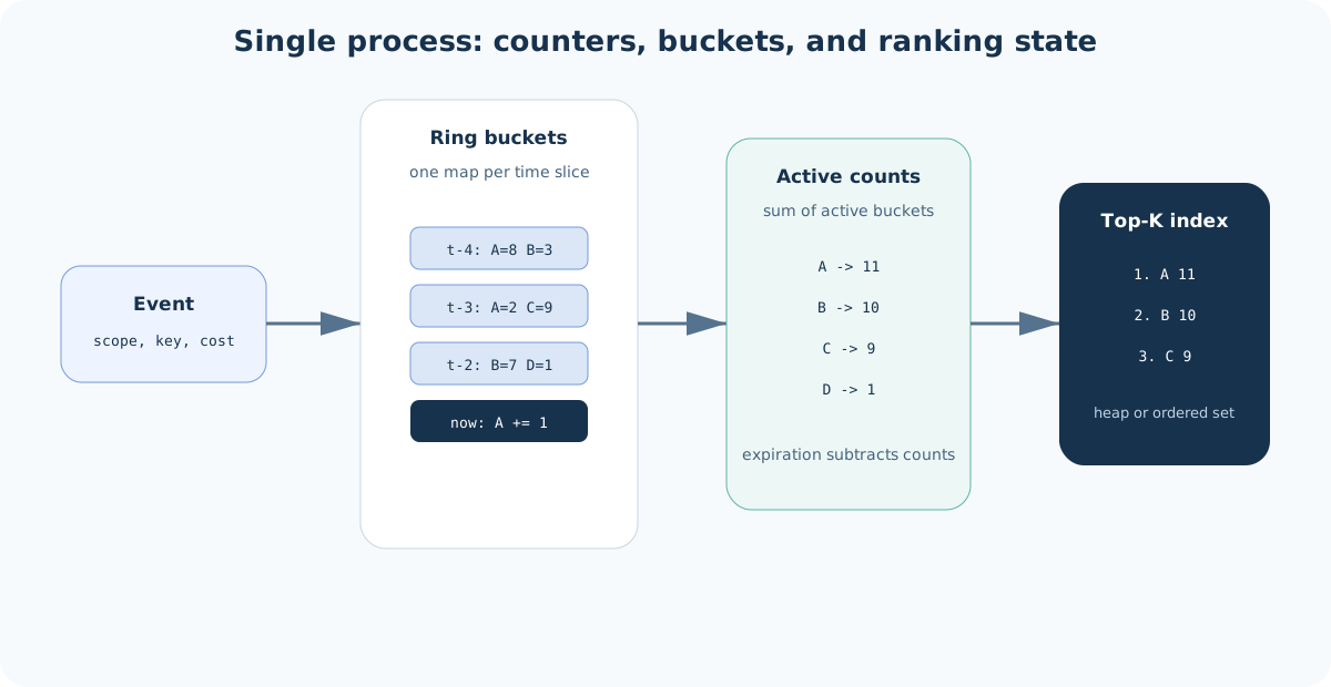
Re-scanning five minutes of raw events every second is expensive. A worker can avoid that by splitting the window into smaller time slices called buckets.
A bucket is a logical time slice. It is not object storage and not a physical container. For readability, the first example uses one-minute buckets:
bucket[10:04] =
  song_8472 -> 300
  song_1931 -> 180
  song_4409 -> 40
This means bucket[10:04] contains counts for events from 10:04:00 through 10:04:59.
Each ranking scope maintains two related structures:
- bucket counts: counts inside one time slice;
- window counts: total counts across all buckets currently inside the sliding window.
Here is how a 3-minute sliding window looks for an active stream scope:
| Bucket | Time Range | song_8472 | song_1931 | song_4409 |
|---|---|---|---|---|
bucket[10:02] | 10:02:00-10:02:59 | 120 | 80 | 30 |
bucket[10:03] | 10:03:00-10:03:59 | 150 | 90 | 50 |
bucket[10:04] | 10:04:00-10:04:59 | 300 | 180 | 40 |
| window_counts | 10:02:00-10:04:59 | 570 | 350 | 120 |
The Top-K ranking is computed from window_counts, not from a single bucket. For K = 2, the current result is:
1. song_8472 -> 570 plays
2. song_1931 -> 350 plays
Buckets exist so the worker can remove old counts without scanning raw events. When a new play for song_8472 arrives during 10:04, the worker updates the current bucket and the running window total:
bucket[10:04][song_8472] += 1
window_counts[song_8472] += 1
When the window advances and bucket[10:02] expires, the worker subtracts that bucket from window_counts:
window_counts[song_8472] -= bucket[10:02][song_8472]
window_counts[song_1931] -= bucket[10:02][song_1931]
window_counts[song_4409] -= bucket[10:02][song_4409]
After subtraction, the old bucket can be cleared and reused:
bucket[10:02].clear()
Production systems often use smaller buckets than this table. A low-latency ranking might use one-second or five-second buckets. The same idea applies: buckets hold per-slice counts; window_counts holds the total for the current window.
A ring buffer is an implementation detail for reusing bucket slots. If the worker keeps 300 one-second buckets for a five-minute window, the next second can reuse the oldest slot after subtracting the old counts from window_counts.
When One Process Breaks
This single-node model is the baseline. A distributed architecture splits, replicates, or approximates this state across multiple nodes.
The single-node model breaks when:
- Write throughput: event volume exceeds one machine’s CPU or network capacity.
- Cardinality: the number of unique entities exceeds available memory.
- Fault tolerance: a process crash can lose in-memory bucket state unless state is checkpointed and replayable.
At scale, the core engineering question changes from a local update problem:
How does one process update its local count tables?
to a distributed ownership problem:
Which worker owns each partition of state, and how is a globally correct Top-K list assembled when workers fail, lag, or restart?
This is the core distributed-systems problem in Top-K heavy hitters. The published list is small, but producing it requires enough distributed state to keep the result fresh, bounded, and recoverable.
2. Data Model
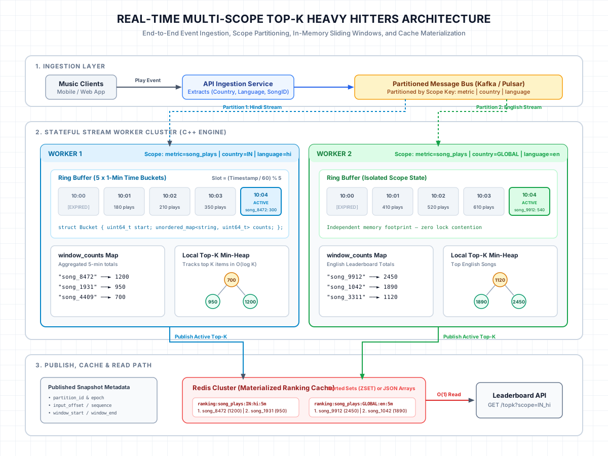
The event should contain the fields required to place the update into the right counter and the right time slice. The running example is a system that maintains the top played Hindi songs in India over the last five minutes.
{
  "event_id": "01J7T4KGMJ9NS8W3B6FMZP4QAJ",
  "event_time": "2026-09-01T19:00:02.481Z",
  "metric": "song_plays",
  "scope": "country=IN|language=hi",
  "key": "song_8472",
  "cost": 1
}
cost = 1 means this event adds one occurrence to the count for song_8472. Weighted Top-K systems can use larger costs, such as bytes uploaded or compute units consumed. The rest of this post assumes cost = 1 unless stated otherwise.
Logical Keys
Top-K aggregation separates the logical identity of a count from the way a worker stores that count.
| Concept | Meaning | Example |
|---|---|---|
| Event key | Entity being ranked | song_8472 |
| Counter key | Exact logical counter being updated | (song_plays, country=IN|language=hi, song_8472) |
| Bucket key | Logical address of one time slice | (song_plays, country=IN|language=hi, bucket=10:04) |
| Ranking key | Served Top-K list | (song_plays, country=IN|language=hi, last_5_minutes) |
The bucket key is the combination of all listed fields. In storage or debug output, the tuple may be encoded as a string:
bucket:song_plays:country=IN|language=hi:10:04
The string format is an encoding choice. The logical key remains:
(metric, scope, bucket_start)
Bucket Storage
Conceptually, each bucket is a map from event key to count:
buckets[bucket_key] = Map<event_key, count>
For the running example:
bucket[song_plays | country=IN|language=hi | 10:04] =
  song_8472 -> 300
  song_1931 -> 180
  song_4409 -> 40
An implementation may flatten the nested map into a key-value table:
(bucket_key, event_key) -> count
Example:
((song_plays, country=IN|language=hi, 10:04), song_8472) -> 300
((song_plays, country=IN|language=hi, 10:04), song_1931) -> 180
((song_plays, country=IN|language=hi, 10:04), song_4409) -> 40
On the internal write path, a worker should not need to concatenate this string on every event. It can use structured fields and local indexes. One possible C++ representation is:
struct Bucket {
  uint64_t start_time_sec;
  std::unordered_map<std::string, uint64_t> counts_by_song_id;
};
Window Counts and Ranking Keys
window_counts is the worker’s current total count per event key across all buckets inside the active window:
window_counts[song_8472] = 1200
window_counts[song_1931] = 950
window_counts[song_4409] = 700
The local Top-K structure ranks window_counts.
The ranking_key identifies the published leaderboard that readers query:
ranking_key = (metric, scope, window_size)
For the running example:
(song_plays, country=IN|language=hi, last_5_minutes)
That key maps to a small sorted result:
1. song_8472 -> 1200
2. song_1931 -> 950
3. song_4409 -> 700
Event Update Flow
For one play event, the worker updates the current bucket, the window total, and the local ranking index:
event_key  = song_8472
bucket_key = (song_plays, country=IN|language=hi, 10:04)

bucket_counts[(bucket_key, event_key)] += 1
window_counts[event_key] += 1
local_top_k.update(event_key, window_counts[event_key])
The read path uses the ranking key:
ranking_key = (song_plays, country=IN|language=hi, last_5_minutes)
Replay Metadata
Because stream workers can lag, crash, or restart, every state snapshot and published summary should carry operational metadata:
owner_idandowner_epoch, identifying the state owner that produced the update;input_offsetorsequence, identifying the stream position processed;window_startandwindow_end, identifying the time range represented;normalization_versionandtopology_version, identifying the rules used.
Without this metadata, retries and failover create ambiguous state. The system may not know whether a published partial ranking is newer, older, duplicated, or produced with incompatible rules.
3. System Architecture
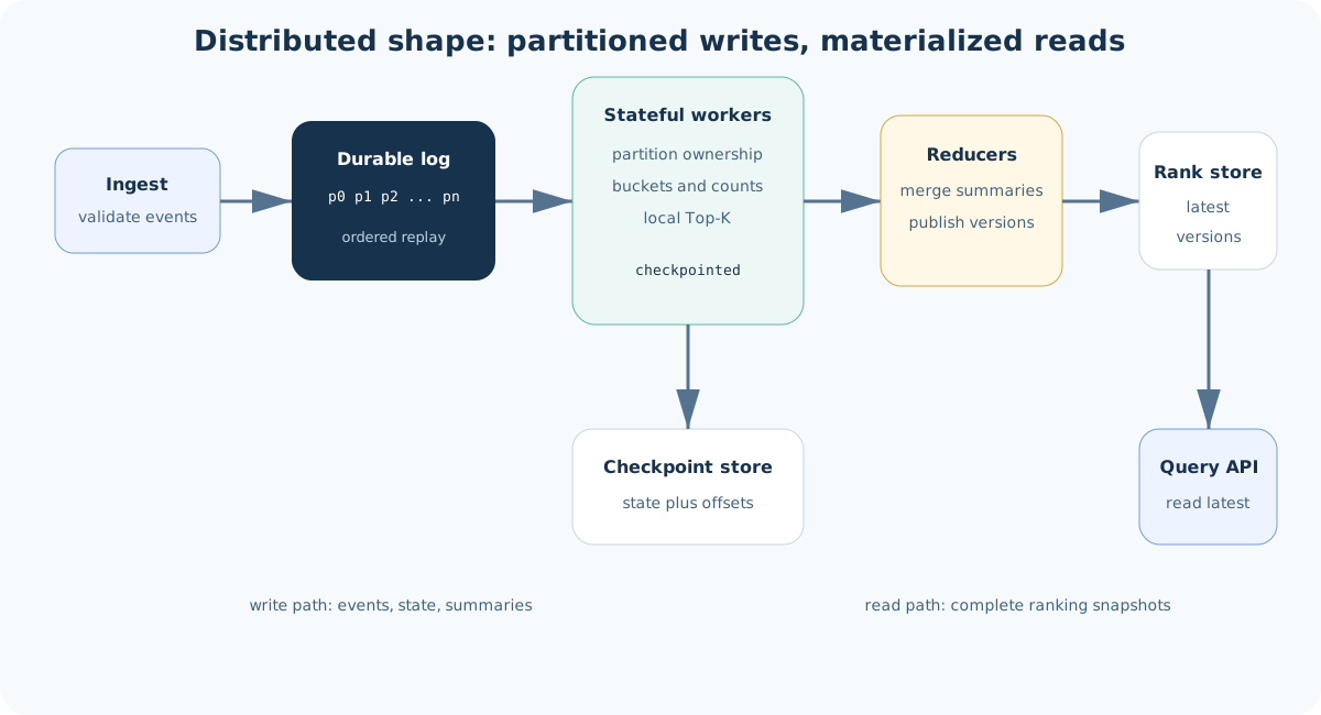
A real-time Top-K service has four kinds of runtime components:
- stateless request/response services;
- a durable message queue;
- long-running stateful workers;
- serving stores for materialized rankings and checkpoints.
The web/API servers handle request traffic. Stream workers maintain Top-K state. Reducers merge worker summaries. The ranking store serves already materialized results.
The deployed shape is:
event producers
    -> load balancer
    -> ingestion API servers
    -> message queue topic
    -> stream worker fleet
    -> reducer fleet
    -> ranking store
    -> query API servers
    -> readers
Ingestion API Servers
The ingestion tier is a stateless web service. It can run as an ECS service, Kubernetes deployment, autoscaled VM group, or serverless HTTP fleet. Its job is to validate and append events; it does not maintain Top-K state.
Typical responsibilities:
- authenticate or trust the upstream service;
- validate required fields;
- attach server receive time;
- normalize or call a normalization library;
- reject malformed or policy-disallowed events;
- append accepted events to the message queue.
The ingestion tier scales horizontally behind a load balancer because each request is independent once the event is written to the queue.
Message Queue Topic
A message queue acts as the durable ingestion buffer for incoming events. The ingestion API writes accepted events to a queue topic, and downstream stream workers subscribe to that topic.
Example topic:
topic = song_play_events
Example event published to the topic:
{
  "event_time": "2026-09-01T10:04:21Z",
  "metric": "song_plays",
  "scope": "country=IN|language=hi",
  "key": "song_8472",
  "cost": 1
}
Several messaging systems can fill this role, including Apache Kafka, AWS Kinesis, Google Cloud Pub/Sub, and Apache Pulsar. The primary requirement is durability. Once an event is written by the message queue, workers can process it, checkpoint progress, and replay from the queue after failure.
Most of these systems divide a topic into partitions:
song_play_events
  partition 0
  partition 1
  partition 2
  ...
Workers subscribe to partitions:
worker A subscribes to partitions 0 and 1
worker B subscribes to partitions 2 and 3
worker C subscribes to partitions 4 and 5
When an API instance accepts an incoming event, it calculates a partition key using a deterministic hash function:
\[\text{partition\_key} = \operatorname{hash}(\text{metric}, \text{scope}, \text{key})\]The queue maps that partition key to a physical partition:
\[\text{target\_partition} = \text{partition\_key} \bmod \text{total\_partitions}\]This keeps all events for one logical key on one partition in the normal case. That property matters because it lets one worker own the count for that key.
Architecture 1: Unified Partitioning
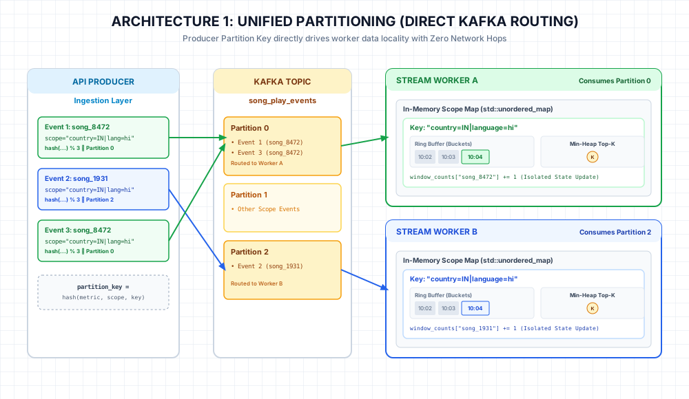
In unified partitioning, routing is handled by the queue’s producer partitioning logic. The ingestion API computes the partition key and writes the event to the selected topic partition.
producer -> queue partition -> stream worker
This design has one queue hop before aggregation. It is simple and low latency, but queue partitioning directly constrains worker parallelism. If one partition or one logical key becomes hot, the worker assigned to that partition receives the concentrated load.
Because a single queue partition can contain events for many scopes, a worker maintains a map from scope to local state:
Worker A state

country=IN|language=hi -> buckets, window_counts, local_top_k
country=US|language=en -> buckets, window_counts, local_top_k
country=BR|language=pt -> buckets, window_counts, local_top_k
Architecture 2: Two-Stage Re-Keying
In two-stage re-keying, the message queue is treated as an ingestion buffer. Routing to stateful Top-K owners happens in a separate worker tier.
API producers
    -> message queue topic
    -> stage 1 ingestion workers
    -> network shuffle
    -> stage 2 state aggregator workers
Stage 1 workers read queue partitions, validate or enrich records if needed, and route events across an internal network connection. Stage 2 workers own state partitions and maintain buckets, window_counts, and local Top-K indexes.
The stage 1 routing function should preserve the same key-ownership rule used by the exact counting path:
\[\text{state\_partition} = \operatorname{hash}(\text{metric}, \text{scope}, \text{key}) \bmod \text{total\_state\_partitions}\] \[\text{target\_aggregator} = \text{routing\_table}[\text{state\_partition}]\]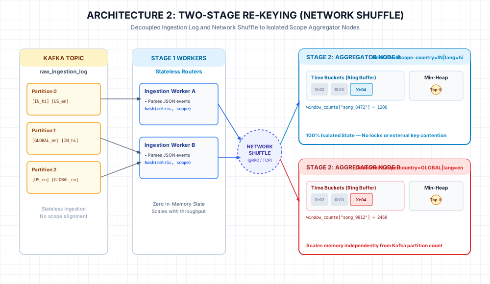
This design adds a network hop, but it allows the message queue partition count and the stateful aggregator fleet size to evolve independently.
Routing Stage 1 to Stage 2
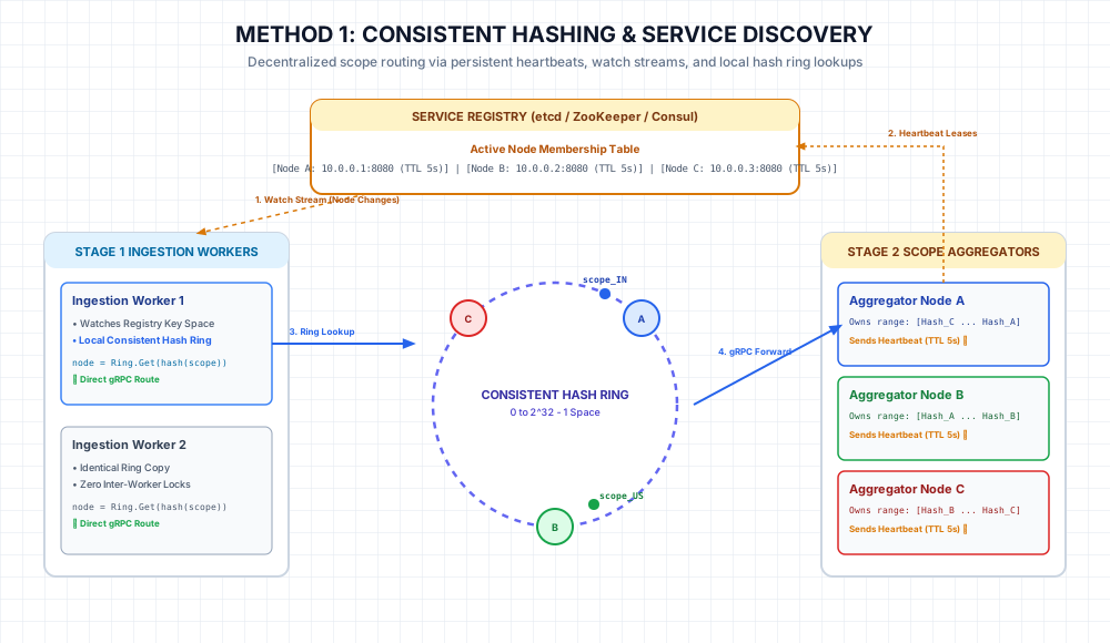
The mapping from stage 1 workers to stage 2 aggregators can be managed with consistent hashing or an explicit control-plane assignment.
Consistent Hashing and Service Discovery
With consistent hashing, stage 2 workers register themselves in a service registry such as ZooKeeper, etcd, or Consul. Stage 1 workers watch the registry, build a local hash ring, and route events locally:
target_node = hash_ring.get_node(hash(metric, scope, key))
If a stage 2 worker fails, its lease expires in the registry. Stage 1 workers receive the membership update and rebuild the ring. Only the state partitions mapped to the failed node move to other nodes.
Centralized Partition Assignments
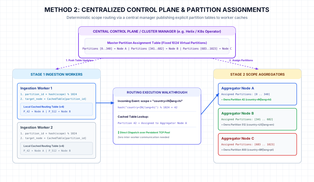
A stricter design uses a control plane to assign virtual partitions to stage 2 workers. Systems such as Apache Helix, a Kubernetes operator, or a custom coordinator can manage this assignment.
virtual_partition = hash(metric, scope, key) % 1024
target_worker = routing_table[virtual_partition]
The controller publishes a versioned routing table to stage 1 workers. Stage 1 workers cache the table and stamp forwarded events with the routing version. This gives operators more predictable ownership and memory placement than a pure hash ring.
Architecture Tradeoffs
| Parameter | Architecture 1: Unified Partitioning | Architecture 2: Two-Stage Re-Keying |
|---|---|---|
| Network Hops | 1 hop: Producer -> Queue -> Worker | 2 hops: Producer -> Queue -> Stage 1 -> Stage 2 |
| Queue Dependency | High: topic partition count directly controls worker parallelism. | Lower: queue partitioning and stateful worker count can scale separately. |
| Traffic Skew Resilience | Limited: a hot key or hot scope can overload its assigned partition worker. | Higher: stage 1 can pre-aggregate, split, or redistribute hot scope traffic. |
| Resource Isolation | Lower: ingestion parsing and state aggregation share the same worker tier. | Higher: ingestion workers and stateful aggregators scale independently. |
| Operational Complexity | Lower: fewer moving parts and fewer internal hops. | Higher: routing, membership, backpressure, and retries exist between stages. |
| Typical Fit | Low-latency systems with controlled skew and bounded partition load. | Systems that need independent scaling of ingestion throughput and state memory. |
Runtime Component Responsibilities
Both architectures use the same runtime roles. The difference is whether queue consumption and state ownership live in one worker tier or in two separate tiers.
Stream Workers
Stream workers are long-running consumers, not web servers. They can run as ECS services, Kubernetes deployments, framework-managed stream tasks, Nomad jobs, or VM processes.
In Architecture 1, the stream worker consumes queue partitions and owns the counting state for those partitions.
In Architecture 2, this responsibility is split:
- Stage 1 workers consume queue partitions and route events.
- Stage 2 aggregators own counting state and maintain local Top-K summaries.
Section 4 describes the state layout inside the stateful owner.
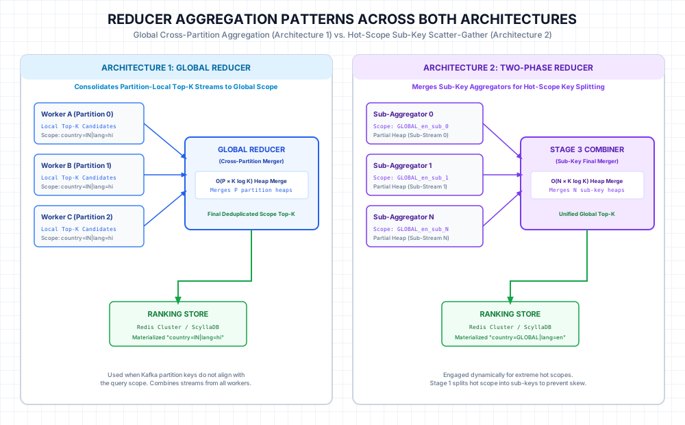
Reducers
Reducers merge local Top-K summaries into one ranking for a ranking_key. They do not read raw events and they do not scan worker memory.
In the normal path, reducers combine one local summary per contributing state owner. If a hot key is split across several owners, reducers also recombine the partial counts for that key before final ranking.
Ranking Store and Query API
The ranking store is optimized for low-latency point reads of pre-materialized Top-K results:
GET /rankings?metric=song_plays&scope=country=IN|language=hi&window=5m
The Query API is stateless. It reads versioned Top-K results from the ranking store and returns them to dashboards, product surfaces, alerting systems, or control loops. It never scans the message queue or polls active stream workers.
Checkpoint and Raw Event Stores
State durability and historical auditing are separate from the real-time serving path.
The checkpoint store persists recovery state for stateful workers and reducers:
state snapshot + queue offset + ownership epoch
Raw event storage keeps immutable incoming events for historical replay, batch auditing, and deterministic rebuilds. The real-time path optimizes for low latency; the offline path verifies or repairs historical results.
4. Distributed Counting Path
Section 3 described two deployment shapes. The counting path is the part that must remain precise in both of them.
The main rule is simple:
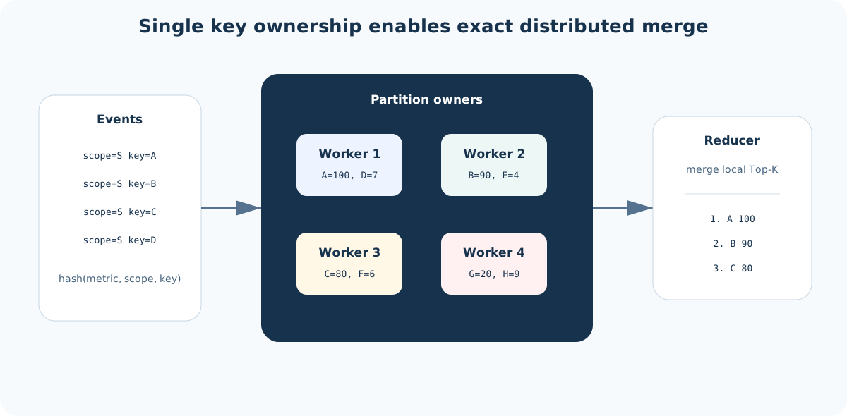
one logical key has one counting owner inside a window
The owner is not necessarily one worker for the whole scope. For a high-traffic scope such as country=IN|language=hi, the scope should usually be spread across many workers by hashing the song ID as part of the ownership key.
Ownership Rule
For exact distributed Top-K, each event for the same logical counter should reach the same stateful owner:
counter_key = (metric, scope, key)
owner = owner_for(counter_key)
For the running example:
counter_key = (song_plays, country=IN|language=hi, song_8472)
owner = state_owner_17
This rule keeps the count for song_8472 in one place. Other songs in the same scope may be owned by other workers:
state_owner_17 -> song_8472, song_1200, song_5521
state_owner_41 -> song_1931, song_4409, song_7712
state_owner_88 -> song_2901, song_3011, song_8120
This is the distinction that matters:
scope ownership:  one worker owns all songs for a scope
key ownership:    many workers own different songs inside the same scope
Scope ownership is easier to reason about, but it overloads quickly when one scope receives most of the traffic. Key ownership is the usual choice for a high-throughput Top-K service because it spreads a hot scope across the worker fleet.
How the Two Architectures Apply Ownership
The local state is the same in both architectures. The difference is how an event reaches the state owner.
| Step | Architecture 1: Unified Partitioning | Architecture 2: Two-Stage Re-Keying |
|---|---|---|
| Queue read | The stateful worker reads its assigned queue partitions directly. | Stage 1 workers read queue partitions first. |
| Owner selection | The queue partition usually determines the owner because producers wrote with hash(metric, scope, key). | Stage 1 computes the state owner from a routing table, virtual partition map, or hash ring. |
| Stateful node | The same worker that reads the queue also maintains buckets and local Top-K. | Stage 2 aggregators maintain buckets and local Top-K. |
| Scaling pressure | Queue partition count and stateful worker parallelism are tightly coupled. | Queue ingestion and stateful aggregation can scale separately. |
| Extra hop | No internal shuffle. | Stage 1 forwards the event to the selected Stage 2 owner. |
In Architecture 1, the event path is:
API server
  -> message queue partition selected by hash(metric, scope, key)
  -> stream worker assigned to that queue partition
  -> local state update
In Architecture 2, the event path is:
API server
  -> message queue topic
  -> Stage 1 ingestion worker
  -> Stage 2 owner selected by hash(metric, scope, key)
  -> local state update
Stage 1 may pre-aggregate a small batch before forwarding, but it should not be the durable owner of sliding-window Top-K state. That state belongs to the stateful worker tier: the unified worker in Architecture 1, or the Stage 2 aggregator in Architecture 2.
Local Update Inside the State Owner
Once the event reaches its state owner, the update is the same as the single-process model. For each active scope and window, the owner maintains:
bucket_counts[(bucket_start, scope, song_id)] -> count in that bucket
window_counts[(scope, song_id)] -> total count inside the current window
local_top_k[scope] -> Top-K over the owned songs for that scope
For one incoming play:
bucket_start = floor(event_time / bucket_size) * bucket_size

bucket_counts[(bucket_start, scope, song_id)] += 1
window_counts[(scope, song_id)] += 1
local_top_k[scope].update(song_id, window_counts[(scope, song_id)])
For one expired bucket:
for each (scope, song_id, count) in expired_bucket:
    window_counts[(scope, song_id)] -= count
    if window_counts[(scope, song_id)] == 0:
        delete window_counts[(scope, song_id)]
    local_top_k[scope].update_or_remove(song_id)
The ranking structure can be an indexed heap, an ordered map, or a lazy heap with compaction. The requirement is not the heap itself. The requirement is that the owner keeps exact window_counts for every song it owns inside the active window. The ranking structure only avoids sorting all owned songs on every publish.
Why Local Top-K Lists Can Be Merged
The reducer does not need every count from every owner when keys are single-owner. It only needs each owner’s local Top-K list for the target scope.
If song_8472 is owned by state_owner_17 and it is not in state_owner_17’s local Top-K, then at least K songs on that same owner have counts greater than or equal to it. Those songs are also valid candidates for the global ranking, so song_8472 cannot be in the global Top-K.
For K = 10 and 200 owners, the reducer merges at most 2,000 candidates for the scope:
candidate_count <= owners_for_scope * K
candidate_count <= 200 * 10
candidate_count <= 2,000
The merge is:
latest local Top-K summaries -> reducer candidate set -> global Top-K
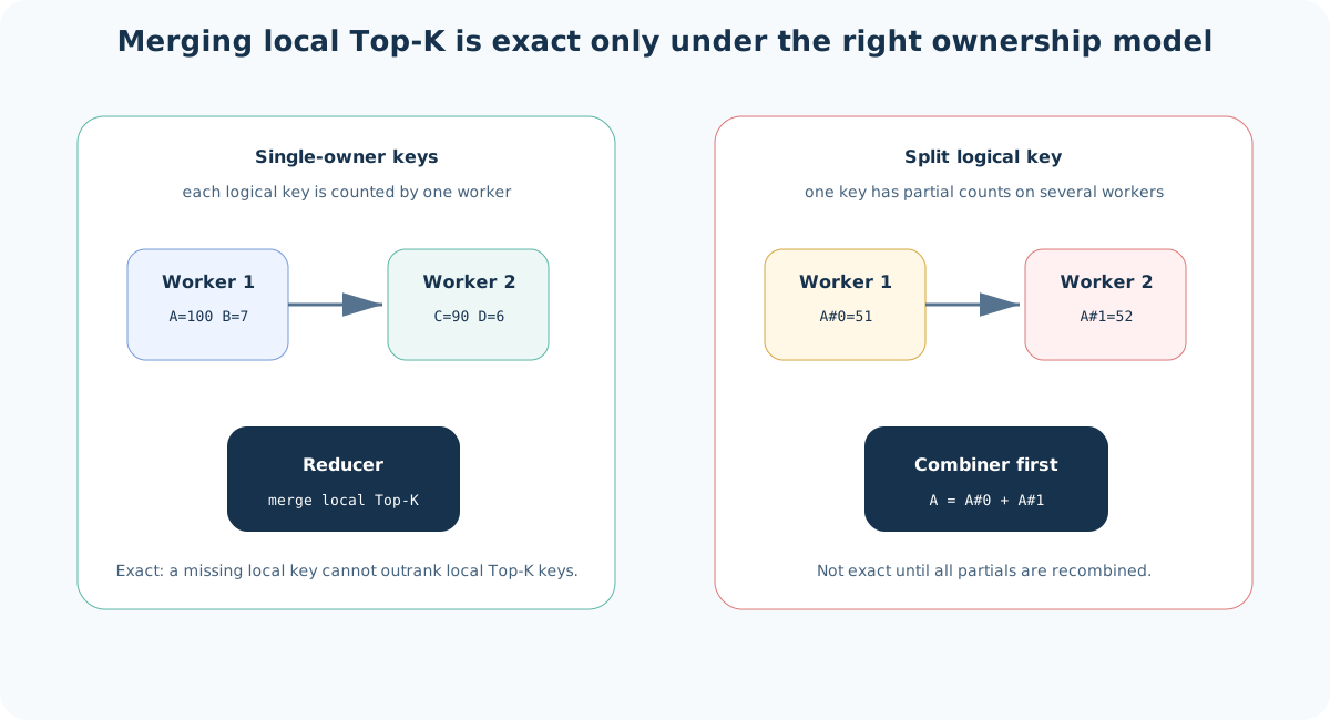
This proof depends on single ownership of each logical key. If a hot song is split across multiple owners, the partial counts must be summed before final ranking. That case is handled separately in the hot-key section.
Publishing Local Summaries
State owners should not publish on every event. At high TPS that would move the bottleneck from local counting to the reducer and ranking store.
A state owner normally publishes:
every publish_interval
or when local Top-K changes materially
or when a bucket expires
The summary identifies the state owner, the ownership epoch, the scope, the window, and the worker’s event-time watermark:
{
  "summary_id": "state-owner-17:epoch-4:seq-98211",
  "owner_id": "state-owner-17",
  "owner_epoch": 4,
  "sequence": 98211,
  "metric": "song_plays",
  "scope": "country=IN|language=hi",
  "window": "5m",
  "watermark": "2026-09-01T19:05:00Z",
  "items": [
    {"key": "song_8472", "count": 992104},
    {"key": "song_1931", "count": 620440}
  ]
}
The reducer keeps the latest accepted summary per (owner_id, scope, window). It ignores summaries with an older sequence or a stale ownership epoch. This makes retries idempotent and protects the final ranking from old workers that continue publishing after failover.
The reducer also tracks completeness. A global ranking for a scope is complete only when all expected owners for that scope have contributed compatible summaries:
candidates = union(latest_summary[owner].items for owner in owners_for_scope)
global_top_k = largest K candidates by count
watermark = min(latest_summary[owner].watermark for owner in owners_for_scope)
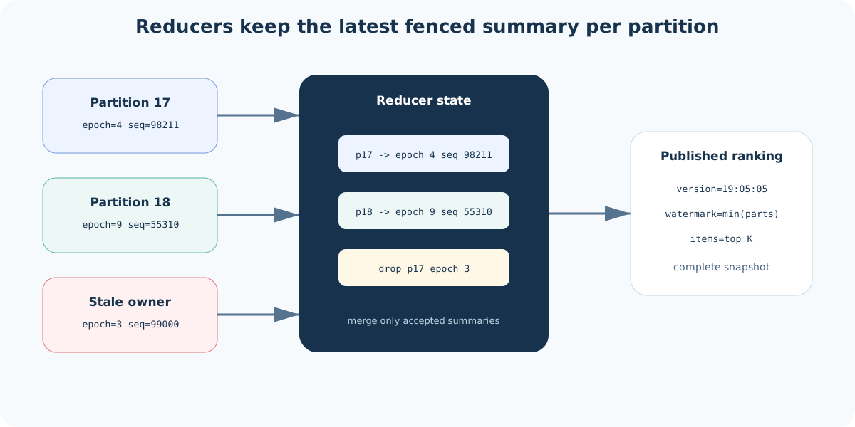
The watermark is the minimum across contributing owners because the global ranking is complete only through the slowest required owner.
Window Advancement Inside Each Owner
The bucket ring described earlier is local to each state owner. If the ranking uses a five-minute window with one-second buckets, each owner keeps 300 bucket slots for the keys it owns:
window_size = 5 minutes
bucket_size = 1 second
bucket_count = 300
The slot is selected by event time:
slot = floor(event_time / bucket_size) % bucket_count
Before a slot is reused for a newer second, the owner subtracts the old bucket from window_counts and repairs local_top_k:
expired_bucket = buckets[slot_for_19_00_00]

for each (scope, song_id, count) in expired_bucket:
    window_counts[(scope, song_id)] -= count
    local_top_k[scope].update_or_remove(song_id)

clear expired_bucket
reuse the slot for 19:05:00
This expiration work is local. Architecture 1 runs it in the queue-consuming worker. Architecture 2 runs it in the Stage 2 state owner. Stage 1 workers do not expire long-lived buckets because they do not own the durable window state.
The owner does not rescan the queue or raw event archive to advance a window. It applies a bounded negative update from the expired bucket.
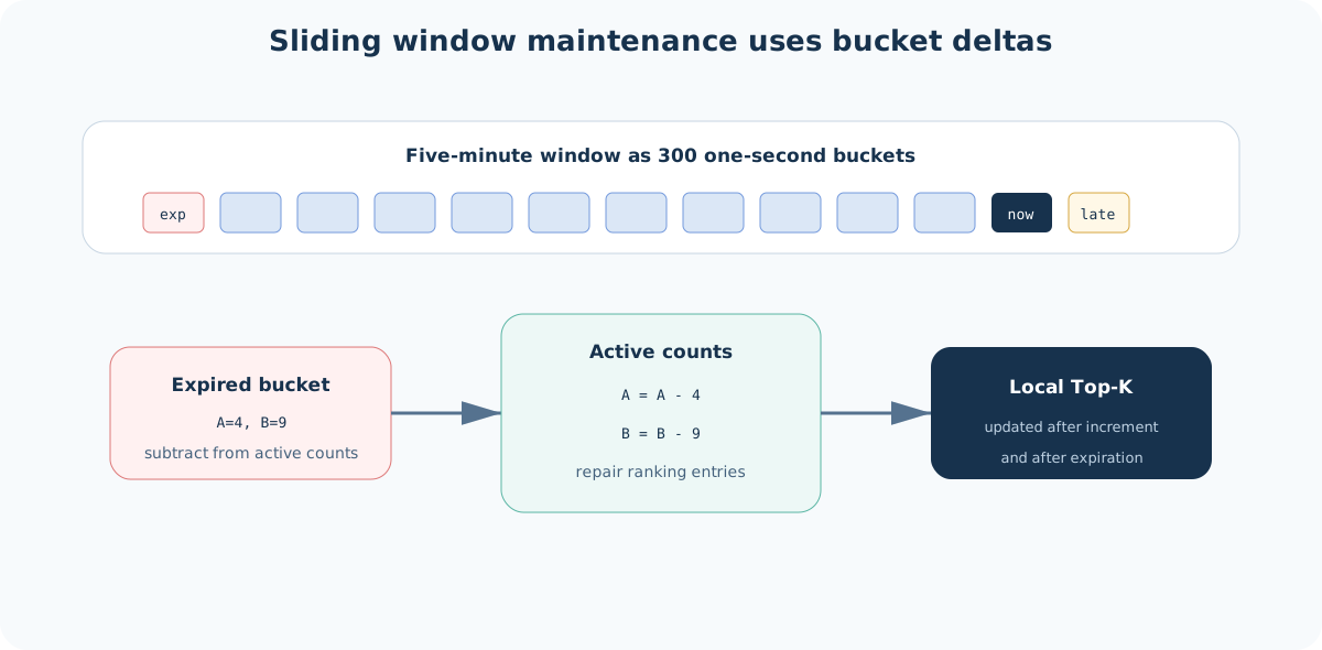
Bucket size remains a tradeoff:
- smaller buckets give fresher expiration and smoother rankings;
- larger buckets reduce memory overhead and expiration work;
- very small buckets can create high metadata overhead for sparse scopes.
Late events require a policy. If the system accepts events up to two minutes late, then recently closed buckets must remain mutable until the watermark passes them. If the event is later than the allowed lateness, either drop it from the real-time ranking or send it to an offline correction path.
The serving API should expose both:
as_of:     when this ranking version was published
watermark: event time through which the ranking is complete
A fresh publish with an old watermark is not a fresh result. It only means the system recently republished stale input.
5. Accuracy and Skew
The previous section describes an exact design under normal ownership rules. Two things can change that model: the keyspace can become too large to keep exactly, or one key can become too hot for a single owner. These are separate problems and should be handled separately.
Exact Counting Versus Bounded Summaries
Exact local Top-K requires exact local counts for all active keys. This is often practical for bounded keyspaces such as known songs, artists, albums, products, or normalized routes. It is harder for open-ended keyspaces such as raw search queries, URLs, error messages, and user-generated labels.
The memory cost is driven by active distinct keys:
memory ~= active_distinct_keys * bytes_per_count_entry
If a worker owns 20 million active keys and each count entry costs 80 to 150 bytes after map overhead and metadata, the worker may need multiple gigabytes for one window family before checkpoints, buckets, and indexes are included.
Approximate summaries reduce memory by accepting controlled error. The common choices are:
| Technique | What it keeps | Merge behavior | Main limitation |
|---|---|---|---|
| Count-Min Sketch | Counter arrays | Add arrays with same parameters | Estimates known keys; does not enumerate keys |
| Space-Saving | Fixed candidate table | Mergeable with care, often used as local candidates | Can overestimate candidates near the cutoff |
| Misra-Gries | Bounded candidate table | Mergeable summaries | Candidate counts need error handling |
| Sampling | Sampled event subset | Merge samples statistically | Weak for rare or bursty keys |
For distributed Top-K, approximation has two separate jobs:
candidate discovery: which keys might be in the top list?
count estimation: what are their counts?
A Count-Min Sketch helps with count estimation but not discovery. A Space-Saving table helps with discovery but may not provide exact counts. A practical approximate design often uses a larger internal candidate set:
visible K = 10
internal candidate size = 100 or 1000
The reducer publishes only K items, but it receives enough candidates to avoid losing keys that are near the boundary.
Approximation should be visible in metadata:
mode = exact | approximate
max_count_error = ...
candidate_size = ...
The system should not represent an approximate rank as exact simply because it is convenient for the API.
Hot Keys
Partitioning by (metric, scope, key) gives one owner per key. That is useful for correctness, but a single heavy key can overload its owner.
Example:
key = song_8472
scope = country=IN|language=hi
traffic = 250,000 plays/second
owner = partition 17
The system may have hundreds of workers, but partition 17 still receives all updates for song_8472.
The common mitigation is key splitting. Once a key is classified as hot, events for that key are distributed across several salts:
partition = hash(metric, scope, key, salt)
salt = hash(event_id) % split_factor
Each salted owner maintains a partial count. A combine stage sums the partial counts for the logical key before the reducer computes the final Top-K.
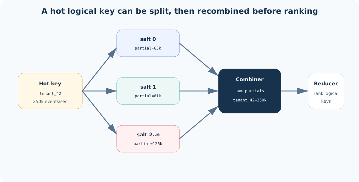
This changes the correctness model. The earlier proof that local Top-K lists are sufficient no longer applies to split keys because the logical key’s count is distributed. The reducer must know the split-key registry and wait for all required partial summaries for that hot key.
Hot-key splitting also needs a transition plan. If a key becomes hot halfway through a sliding window, some buckets may contain unsplit counts and newer buckets may contain salted counts. The ranking layer must sum both forms until the unsplit buckets age out.
logical_count(key) =
    unsplit_count(key)
  + sum(partial_count(key, salt) for active salts)
The split registry should be versioned and included in event metadata or worker configuration. Otherwise replay can route old events differently from the original processing path.
Reducer State
Reducers are stateful. For each ranking key they keep:
latest_summary_by_partition
latest_summary_by_hot_key_partial
current_candidate_counts
current_global_top_k
published_version
watermark_by_partition
The reducer does not need all raw event counts when keys are single-owner. It needs the latest local summaries. For split hot keys, it also needs enough partial information to reconstruct the logical key count.
Reducers can be partitioned by ranking key:
reducer_partition = hash(metric, scope, window_size)
This keeps all summaries for one served ranking on one reducer. If one scope becomes too hot at the reducer layer, use a tree:
worker summaries -> regional reducers -> global reducer -> ranking store
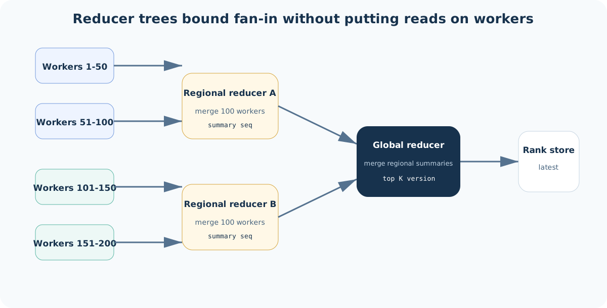
Each level should publish versioned summaries in the same way workers do. This keeps the merge protocol uniform and makes recovery simpler.
6. Resiliency
The ranking is useful only if failures do not silently corrupt it. The main resiliency rule is to make every visible result versioned, complete for a known watermark, and tied to the worker epochs that produced it.
Ranking Publication
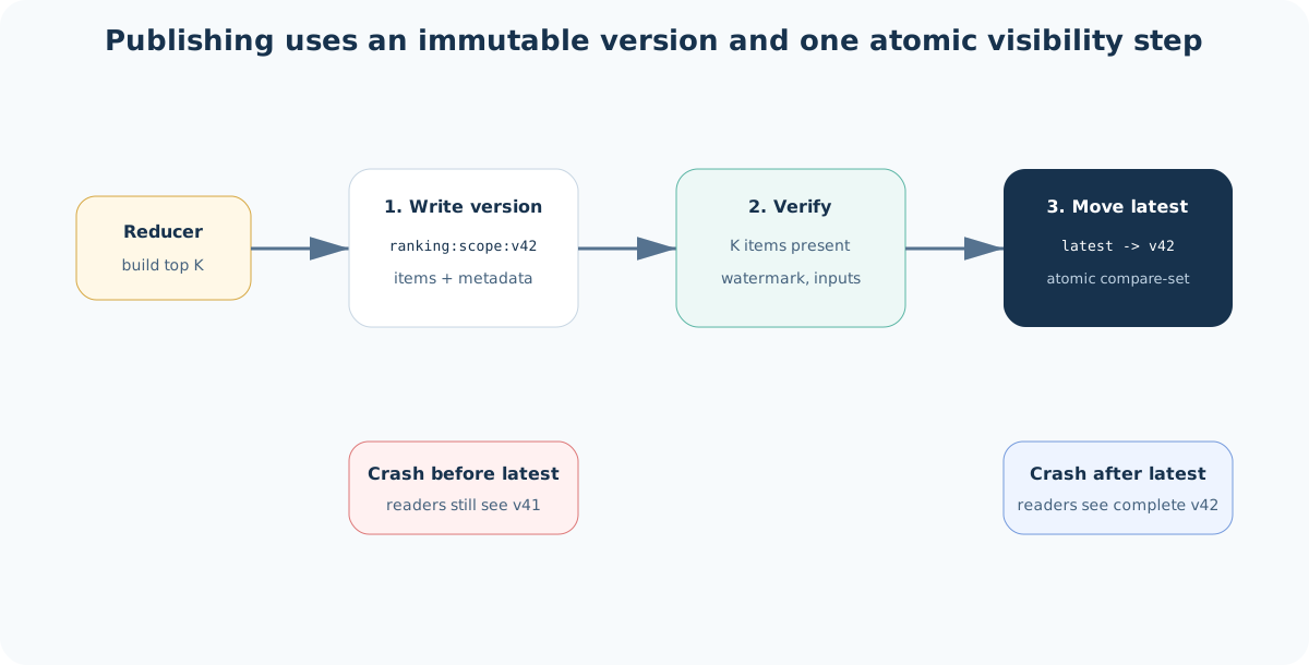
The published ranking should be immutable.
write ranking:{metric}:{scope}:{window}:{version}
verify item count and metadata
atomically update ranking:{metric}:{scope}:{window}:latest -> version
expire older versions after retention
Readers follow the latest pointer and receive one complete ranking version. They should not observe a ranking while it is being written.
The ranking record should include:
items:       rank, key, count, optional error
as_of:       publication time
watermark:   minimum contributing event-time watermark
mode:        exact or approximate
version:     monotonically increasing ranking version
input_range: optional partition offsets or summary sequences
The input_range is useful during incidents. It answers which queue offsets or summary sequences contributed to a visible result.
Worker Failure and Replay
A stateful worker can fail at any time. Recovery needs three pieces:
durable input queue
checkpointed local state
committed input offset
The checkpoint contains count maps, bucket state, ranking state, watermarks, and any approximate summaries. The committed offset records the point in the input queue represented by that checkpoint.
On restart:
load latest checkpoint
seek input partitions to checkpoint offset
replay events after that offset
resume publishing with a new partition epoch
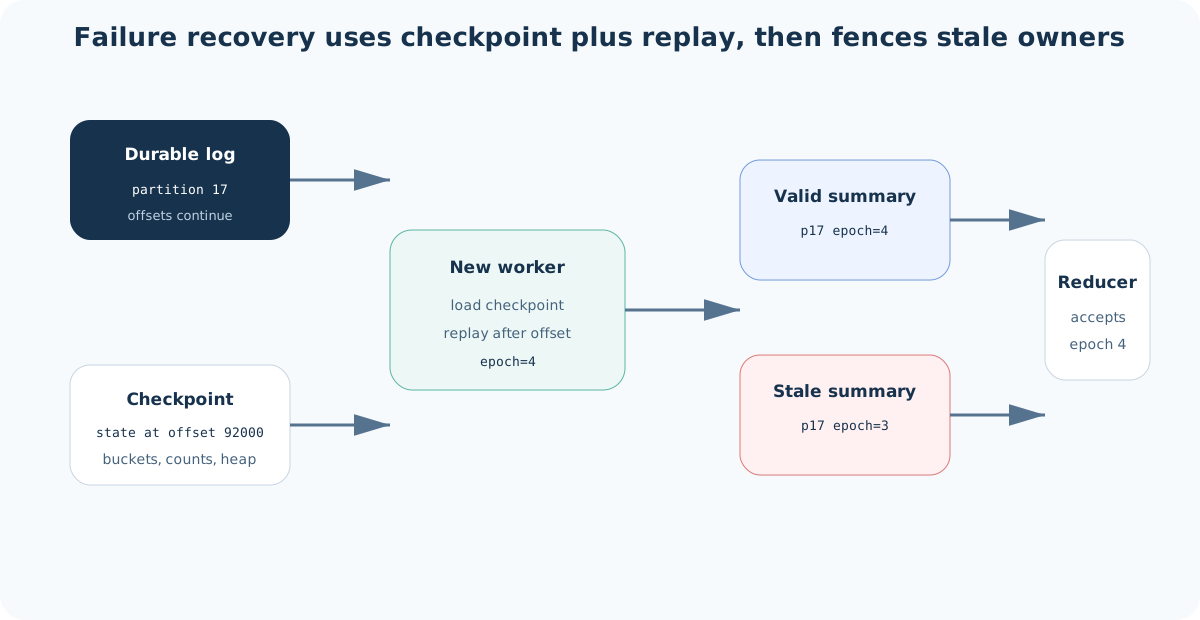
The partition epoch matters. During failover, the old worker may still be alive but partition ownership has moved. If both old and new workers publish summaries, the reducer must accept only the active epoch.
accept summary if owner_epoch == current_owner_epoch
ignore summary if owner_epoch < current_owner_epoch
reject or quarantine summary if owner_epoch > known_owner_epoch
This fencing rule prevents stale owners from corrupting the published Top-K.
Reducer Failure
A reducer can recover in several ways.
The simplest method is to rebuild from the latest summaries published by all workers. This requires workers, or an intermediate summary topic, to retain their latest summary for each active ranking key.
A stronger method gives the reducer its own durable state-change topic:
summary update -> reducer state update -> reducer state-change topic -> publish
On restart, the reducer loads its checkpoint and replays summary updates after the checkpoint. This mirrors the worker recovery path.
Reducer recovery should be tested with partial publish failures. If the reducer crashes after writing a ranking version but before advancing the latest pointer, readers continue seeing the old version. If it crashes after advancing the pointer, the version is already complete. The atomic pointer is the commit point for serving.
Duplicate Events and Exactly-Once Claims
Most real systems are at least once at one or more boundaries. Producers retry. Queue clients retry. Workers restart after checkpointing. Publishers retry summary writes.
There are two defensible approaches.
The first approach makes event processing idempotent. Keep a bounded dedupe set keyed by event_id per partition and window. This is expensive but useful when counts drive enforcement or billing-like decisions.
The second approach accepts that duplicate events can enter real-time Top-K and corrects through offline jobs. This can be acceptable for exploratory dashboards, but the duplicate rate should be measured and visible.
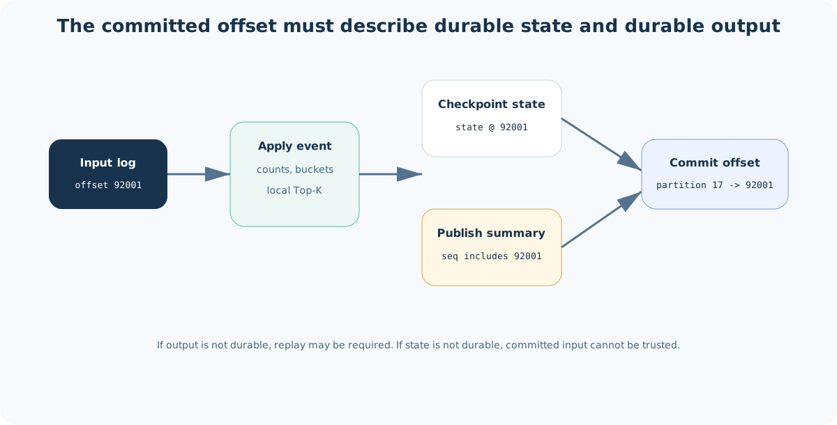
Exactly-once stream processing frameworks can reduce application complexity, but the design should still name the commit point:
input offset is committed only after state checkpoint and output summary are durable
If the system cannot state this boundary, the exactly-once claim is not precise enough for debugging.
Backpressure and Staleness
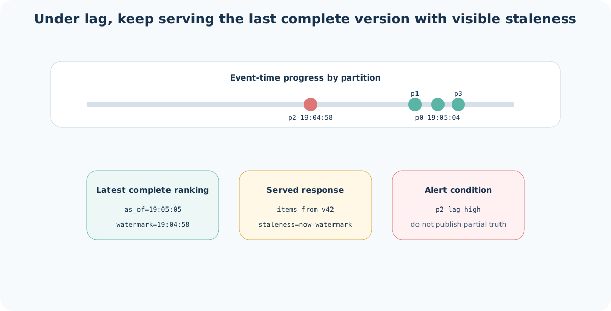
A high-TPS Top-K system should degrade by becoming stale, not by serving partially merged rankings as if they were complete.
Backpressure can appear in several places:
- ingestion cannot append to the queue fast enough;
- one queue partition accumulates lag;
- workers cannot update state fast enough;
- bucket expiration takes too long;
- reducers cannot merge summaries fast enough;
- the ranking store throttles writes.
The serving layer should continue returning the last complete ranking with metadata:
as_of = 19:05:05
watermark = 19:04:58
staleness = now - watermark
Callers can decide whether that result is usable. Internally, alerts should be based on watermark lag per ranking key, not only CPU or queue depth. A system with low CPU and an old watermark is still failing its freshness contract.
Regional Failure
Multi-region Top-K can be built in two ways.
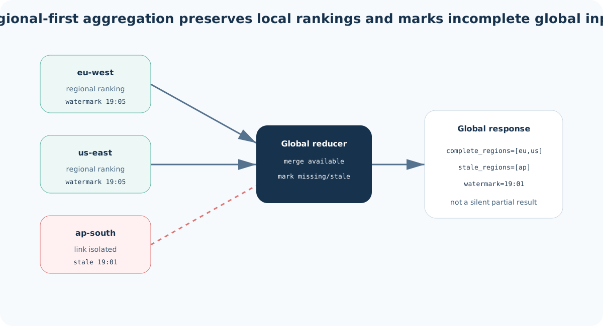
In a regional-first design, each region maintains local rankings and publishes regional summaries. A global reducer merges regional summaries.
region workers -> regional reducer -> global reducer
This keeps regional results available when cross-region links fail. The global result may become incomplete. The global watermark should make that visible.
In a global-stream design, all events replicate into one logical stream before aggregation. This gives a simpler global ordering model but adds dependency on cross-region replication and can increase latency.
For operational heavy hitters such as hot songs, hot search terms, or hot API routes, regional-first is often useful because incidents are frequently regional. For strict global counts, the real-time ranking should be paired with an offline reconciliation path.
During a regional outage, avoid silently mixing complete and incomplete input. A global ranking can be marked:
complete_regions = [eu-west, us-east]
missing_regions = [ap-south]
watermark = min(watermark of complete regions)
This is better than publishing a precise-looking global list that excludes one region.
7. Operations
The operational design is the part that keeps the system understandable after deployment. It defines who owns a partition, which rules workers are using, where state is stored, and how freshness is measured.
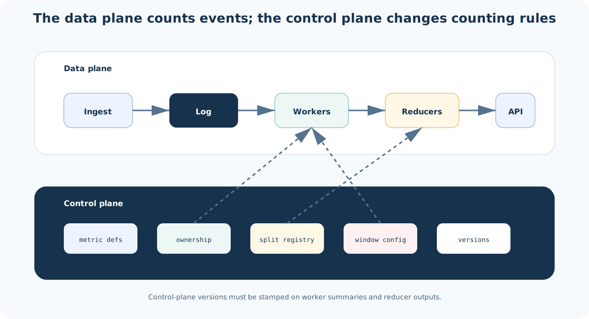
Control Plane
The data plane processes events. The control plane manages the rules used by the data plane.
Control-plane state includes:
- metric definitions;
- normalization versions;
- allowed scopes;
- partition assignments;
- worker ownership epochs;
- hot-key split registry;
- window definitions;
- approximate-summary parameters;
- publication cadence;
- retention policy.
The control plane should be versioned. Workers should stamp outputs with the versions they used. Reducers should not merge summaries produced with incompatible versions unless the merge rule explicitly supports it.
For example, if song identity normalization changes from display title to a canonical song ID, the counts are no longer comparable:
song="Kesariya"
song="Kesariya - From Brahmastra"
may become:
song_id=song_8472
The system should either start a new ranking version family or run a migration that makes the change explicit.
Storage Choices
The hot state usually lives close to the stream workers.
Worker state can be stored in embedded RocksDB, an in-memory map with periodic snapshots, or a framework-managed state store. The choice depends on state size and recovery expectations.
Reducers need less state than workers but have stricter publication semantics. Their state can also be checkpointed locally and written to a durable state-change topic.
The ranking store should optimize reads:
GET latest ranking for metric + scope + window
Redis, DynamoDB, Cassandra, FoundationDB, or a relational table can all work depending on the surrounding system. The store should support atomic latest pointer updates or equivalent compare-and-set semantics.
Raw events should be retained separately in object storage or a long-retention queue when rebuilds, audits, or offline validation are required.
Observability
The main health signal is not the size of the final list. It is whether every required partition is contributing fresh, compatible input to that list.
Track:
- ingest events per second by metric, scope, and region;
- queue append latency and partition lag;
- active distinct keys per worker;
- worker state size and checkpoint duration;
- bucket expiration duration;
- local Top-K publish rate and payload size;
- reducer fan-in per ranking key;
- stale or missing partition summaries;
- global watermark lag;
- ranking publication failures;
- latest-pointer update failures;
- hot-key split count and partial-summary completeness;
- replay duration after worker restart;
- exact-vs-approximate error on sampled windows.
For approximate Top-K, track rank overlap with exact offline results:
overlap = size(real_time_top_k ∩ exact_top_k) / K
Count error alone is not enough. A system can have small count error and still publish an unstable rank order near the cutoff.
Failure Matrix
| Failure | Expected behavior |
|---|---|
| Worker crash | New owner restores checkpoint, replays queue events, publishes with a new epoch. |
| Old worker resumes | Reducer ignores summaries from the stale epoch. |
| Reducer crash | Reducer reloads checkpoint or rebuilds from retained latest summaries. |
| Ranking store write fails | Readers continue using the previous complete version. |
| Latest pointer update fails | New version remains invisible until retry succeeds. |
| One partition lags | Global watermark stops advancing; result is served as stale. |
| Hot key overloads owner | Control plane enables salted split; reducer recombines partial counts. |
| Region isolated | Regional ranking continues; global ranking marks missing or stale regions. |
| Bad normalization deploy | Outputs carry normalization version; reducers reject incompatible summaries. |
| Backfill replays old events | Backfill writes to a separate rebuild path or uses idempotent window versions. |
This matrix is part of the design, not an operations appendix. Top-K systems are often used during incidents. Their own failure modes must be visible.
8. Reference Design
A practical high-throughput exact design for bounded keyspaces looks like this:
- Events are validated and written to a durable partitioned message queue.
- Partitions are assigned by
hash(metric, scope, key). - Each worker owns a set of partitions under a fenced epoch.
- Workers maintain exact window counts, bucket counts, and local Top-K per scope.
- Workers checkpoint state and committed offsets.
- Workers publish versioned local Top-K summaries at a fixed cadence.
- Reducers keep the latest summary per state owner and merge candidates.
- Reducers publish immutable ranking versions and atomically advance latest pointers.
- The query API reads the latest complete ranking version.
- Offline jobs validate selected windows and rebuild when needed.
- The control plane manages partition ownership, hot-key splits, and compatible configuration versions.
For unbounded keyspaces, replace exact local counts with bounded summaries where necessary, but keep the same ownership, publication, recovery, and serving structure. Approximation changes the accuracy contract; it should not remove versioning, watermarks, fencing, or replay.
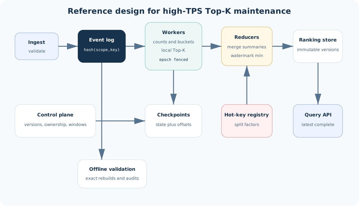
The system is correct only relative to the contract it publishes. For exact mode, the contract depends on single ownership of each logical key or complete recombination of split keys. For approximate mode, the contract depends on the summary algorithm and candidate size. For both modes, resiliency depends on durable input, checkpointed state, fenced ownership, idempotent summaries, atomic publication, and visible watermarks.
Leave a Comment