Inside Sharding: Partition Maps, Consistent Hashing, Rebalancing, and Hotspots
Published:
1. Introduction
The Moment One Storage Node Is Not Enough
A single storage node has a simple ownership model:
every key -> one node
The node owns the complete keyspace, so every read and write has an obvious destination. Local indexes can cover all data. Transactions do not cross a network boundary. Backups, compaction, and recovery operate on one storage engine.
That model stops being appropriate when the workload exceeds one node’s useful limits:
- the retained dataset no longer fits with operational headroom;
- read or write throughput saturates CPU, storage, or network;
- maintenance and recovery take too long;
- one tenant or workload must be isolated;
- geographic placement requires data to live in several locations.
Sharding divides the keyspace into independently owned pieces so capacity can grow across machines:
keyspace
  -> shard S1
  -> shard S2
  -> shard S3
The division creates a new distributed-systems problem:
Given a key and a changing set of shards, which shard owns the key now, and how can ownership change without losing or duplicating data?
That question is the core of sharding.
Sharding Is More Than Hashing
Choosing a hash function is only one part of the design. A complete sharded system needs to answer:
- What is the partition key?
- Is ownership based on ranges, hashes, slots, or a directory?
- Where is the partition map stored?
- How do clients learn and refresh that map?
- How are replicas placed inside each shard?
- What happens when one shard becomes hot?
- How is a shard split, moved, or merged while writes continue?
- How are stale routers rejected or redirected?
- What guarantees exist for cross-shard reads and transactions?
- How does the system recover when migration fails halfway through?
This article develops the system from the placement function through live rebalancing and operational failure.
2. A Precise Model
Partition, Shard, Replica, and Node
These terms are often used interchangeably even though they describe different things.
A partition is a logical subset of the data. It may be a key range, hash range, slot, tablet, or bucket.
A shard is an independently managed unit of ownership and scaling. In many systems a shard contains one or more partitions and has its own replication group.
A replica is an additional copy of a shard’s data.
A node is a process or machine that may host several shard replicas.
For example:
logical shard S7
  leader replica  -> node A
  follower replica -> node B
  follower replica -> node C
Sharding divides data. Replication copies each division. A system can be:
sharded but not replicated
replicated but not sharded
both sharded and replicated
Production databases normally combine both.
The Placement Function
Let:
K = set of application keys
P = set of logical partitions
N = set of storage nodes
Sharding defines two mappings:
partition_for: K -> P
placement_for: P -> ordered replicas in N
The first mapping decides the logical owner. The second decides where copies of that owner run.
Separating them is powerful. A partition can move from node A to node D without changing which keys belong to the partition.
Four Core Invariants
At any committed metadata version, a useful partition map should provide:
Coverage: every valid key maps to a partition.
Unique primary ownership: one authoritative shard or replication group is responsible for ordering writes to that partition.
Deterministic routing: routers using the same metadata version compute or look up the same destination.
Versioned change: an ownership transition has an order, so stale and current routing decisions can be distinguished.
Balance and bounded movement are desired properties, but the four invariants are correctness properties.
Measuring Balance and Movement
For load L_i assigned to shard i, a simple skew measure is:
skew = maximum shard load / average shard load
A perfectly balanced model has skew 1.0. Real systems balance several dimensions separately:
stored bytes
reads per second
writes per second
CPU time
network bandwidth
tenant concentration
When membership changes from placement function R_old to R_new, the movement fraction is:
movement =
  keys whose owner changes / total keys
Low movement reduces cache churn and migration work. It does not guarantee balanced traffic.
3. Routing Architecture
The Data Path
Every operation needs a routing decision before local storage can execute it:
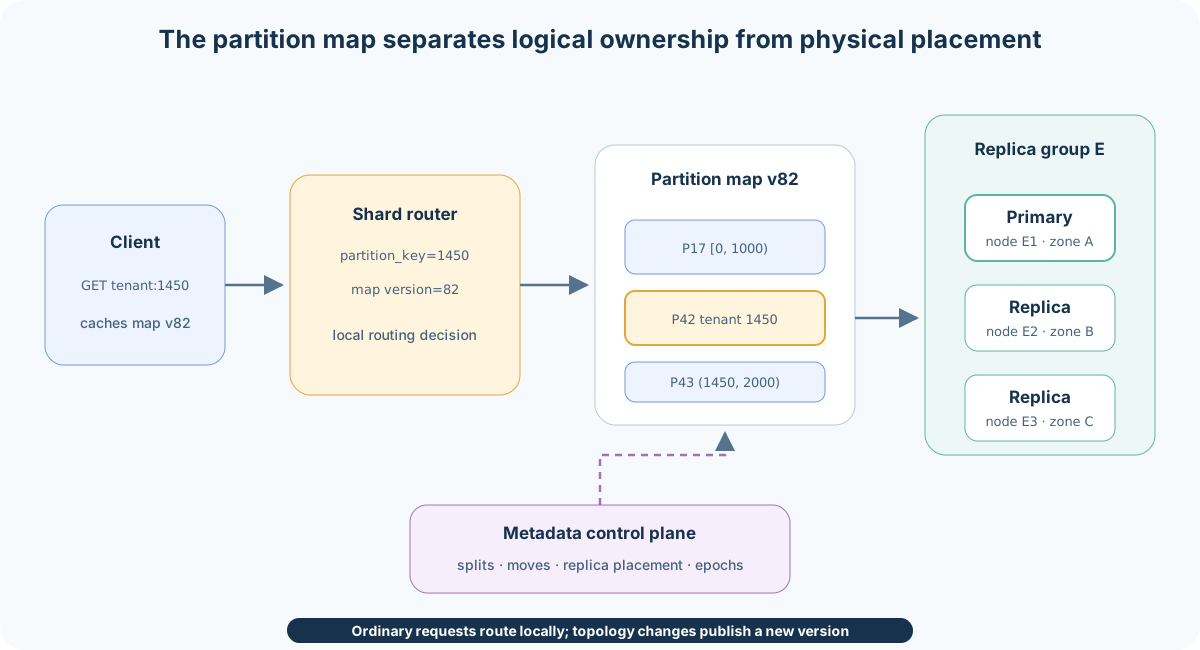
The steady-state path is:
application key
  -> extract partition key
  -> compute or look up logical partition
  -> find current replica group
  -> send operation to the appropriate replica
The destination may be selected by:
- a database-aware client;
- a stateless routing proxy;
- a coordinator node inside the database;
- a metadata service consulted and cached by clients.
The common path should normally use local cached metadata rather than synchronously consulting a control-plane service for every request.
The Control Plane
The control plane manages:
- partition boundaries or tokens;
- shard-to-node placement;
- replica roles;
- split, merge, and migration operations;
- health and failure-domain constraints;
- metadata epochs or versions.
Its output is a partition-map snapshot:
map version 42

[-infinity, customer:4000) -> shard S1 -> nodes A, B, C
[customer:4000, customer:8000) -> shard S2 -> nodes D, E, F
[customer:8000, +infinity) -> shard S3 -> nodes G, H, I
The data plane consumes that snapshot. This is the same architectural separation seen in load balancers and distributed caches: coordination changes the map; ordinary requests use it locally.
Client-Side, Proxy, and Coordinator Routing
Client-side routing gives the shortest path and removes a proxy hop. Clients must implement metadata refresh, retries, and topology-change behavior.
Proxy routing centralizes policy and client compatibility. The proxy fleet becomes another capacity and availability layer.
Coordinator routing lets a client contact any database node. The contacted node forwards or coordinates the operation, simplifying the client but adding an internal hop when it is not the owner.
No choice removes routing metadata. It only changes who owns its complexity.
4. Choosing the Partition Key
The Partition Key Defines Locality
The partition key determines which data can live and execute together. Consider events keyed as:
(tenant_id, event_time, event_id)
If the partition key is only tenant_id, all events for one tenant are co-located and time-range queries are efficient within that tenant. A dominant tenant can create an oversized or overloaded partition.
If the partition key is:
(tenant_id, time_bucket)
the tenant is spread across time buckets. Writes and retention become easier to distribute, but a long time-range query fans out across several partitions.
Partition-key design chooses which operation is local and which operation must coordinate.
Cardinality
A partition key needs enough distinct values to create useful parallelism.
Bad candidates often include:
country
status
boolean flag
current date
If there are three status values, the system cannot distribute that dimension across hundreds of shards without adding another key component.
Stability
Changing a partition key usually requires moving or rewriting data. Prefer attributes that do not change during the record’s lifetime.
For example, sharding user records by current country creates migration work when users move and makes identity lookups depend on mutable state. Sharding by stable user ID avoids that ownership change.
Locality Versus Distribution
Two objectives compete:
put related data together
spread load evenly
Maximum locality can create hotspots. Maximum randomization can turn every useful query into fanout. Good partition keys preserve the locality required by dominant operations while creating enough independent units to distribute load.
5. Range Partitioning
Ordered Boundaries
Range partitioning assigns contiguous key intervals:
[-infinity, 1000) -> P1
[1000, 2000)      -> P2
[2000, +infinity) -> P3
A router stores sorted upper boundaries and performs a binary search:
from bisect import bisect_right


class RangeMap:
    def __init__(self, upper_bounds, partitions):
        if len(partitions) != len(upper_bounds) + 1:
            raise ValueError("one more partition than boundaries")

        self.upper_bounds = list(upper_bounds)
        self.partitions = list(partitions)

    def locate(self, key):
        index = bisect_right(self.upper_bounds, key)
        return self.partitions[index]


owners = RangeMap(
    upper_bounds=[1_000, 2_000],
    partitions=["P1", "P2", "P3"],
)

assert owners.locate(400) == "P1"
assert owners.locate(1_500) == "P2"
assert owners.locate(9_000) == "P3"
With p partitions, lookup is O(log p).
Why Ranges Are Useful
Related keys remain adjacent. A query:
customer_id from 4000 through 4999
touches the small set of partitions overlapping that interval. Storage within each partition can remain sorted, making range scans efficient.
Range partitioning also supports explicit split points. An oversized partition:
[1000, 2000)
can become:
[1000, 1500)
[1500, 2000)
The Moving-Frontier Hotspot
Monotonically increasing keys concentrate new writes at the end:
timestamp
auto-incrementing ID
lexicographically ordered event sequence
The newest range receives nearly all writes while older ranges are mostly idle.
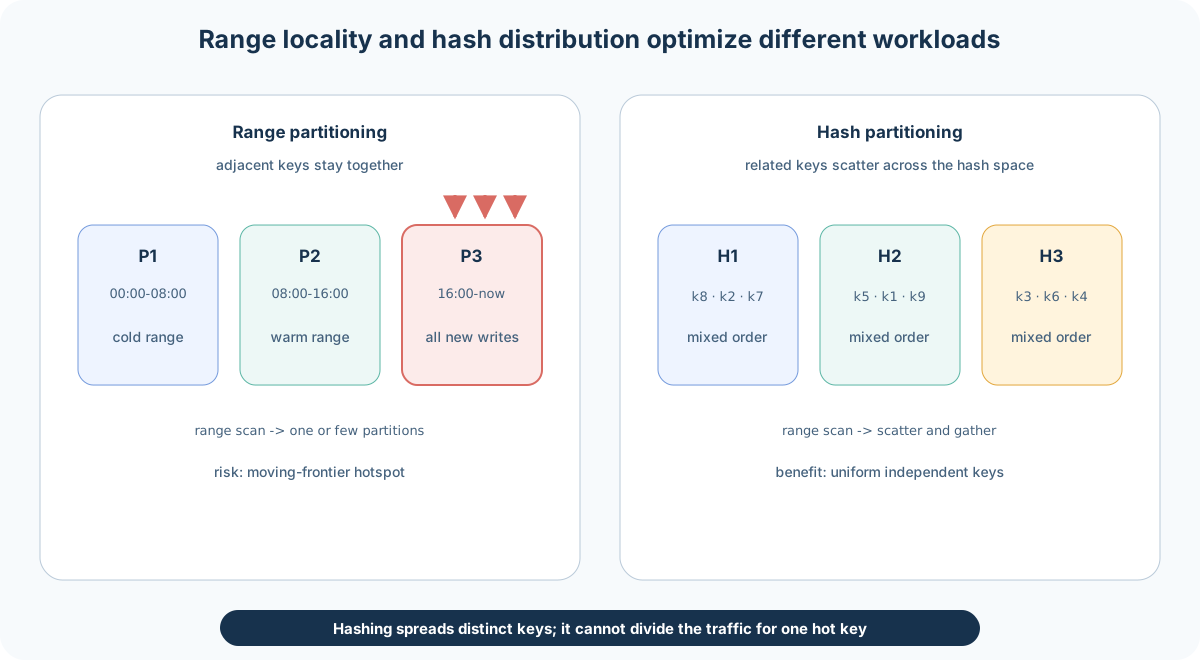
Mitigations include:
- prefixing time with a stable entity ID;
- adding a write bucket;
- splitting the active range more aggressively;
- using a hash prefix while retaining time order inside each prefix.
Each mitigation increases read fanout for queries that do not know the prefix.
6. Hash Partitioning
Hash First, Then Assign
Hash partitioning transforms the partition key into a uniform-looking value:
token = hash(partition_key)
partition = owner(token)
Related input keys normally produce unrelated tokens. This distributes keys more evenly than their natural order.
A fixed-slot design might use:
slot = hash(key) mod 16,384
partition = slot_map[slot]
The key-to-slot function remains fixed while slots move between shards.
What Hashing Gives Up
Hash order is not application order. A query over:
timestamps from 12:00 through 13:00
cannot locate a small hash interval unless another key component first narrows the partition. The query may fan out across every shard.
This is why many databases separate:
partition key -> hashed for distribution
clustering key -> sorted within the partition
For:
PRIMARY KEY ((user_id), event_time, event_id)
user_id selects the partition. event_time and event_id order rows inside it. Per-user time-range queries stay local, but a single very active user can still become hot.
Uniform Keys Do Not Mean Uniform Load
A good hash function can distribute a million distinct keys evenly while one key receives half the traffic:
50% of requests -> celebrity:42
50% of requests -> 999,999 other keys
The celebrity key has only one hash value and therefore one owner. Hashing solves key-distribution skew, not popularity skew.
7. Why Modulo Hashing Breaks Under Change
The Simple Rule
The simplest mapping is:
owner = hash(key) mod number_of_shards
With four shards:
hash(k1) mod 4 -> S0
hash(k2) mod 4 -> S1
hash(k3) mod 4 -> S2
hash(k4) mod 4 -> S3
The problem appears when the shard count changes. After adding a fifth shard:
owner = hash(key) mod 5
Most remainders change. For large independent hashes, only about:
1 / new_shard_count
remain on the same numeric remainder by coincidence when moving from n to n + 1. The majority of keys move.
Why Movement Matters
Mass remapping creates:
- bulk data transfer;
- cold caches;
- duplicate or missing reads during transition;
- extra network and storage load;
- long recovery time;
- operational risk proportional to the entire dataset.
Modulo hashing is reasonable when membership is fixed or when the stored state is disposable. It is usually a poor ownership function for a large persistent dataset whose shard count changes.
8. Consistent Hashing
A Shared Token Space
Consistent hashing maps both keys and shard tokens into a circular hash space:
0 -------------------------------------- 2^64 - 1
^                                          |
|__________________________________________|
A key belongs to the first shard token encountered clockwise.
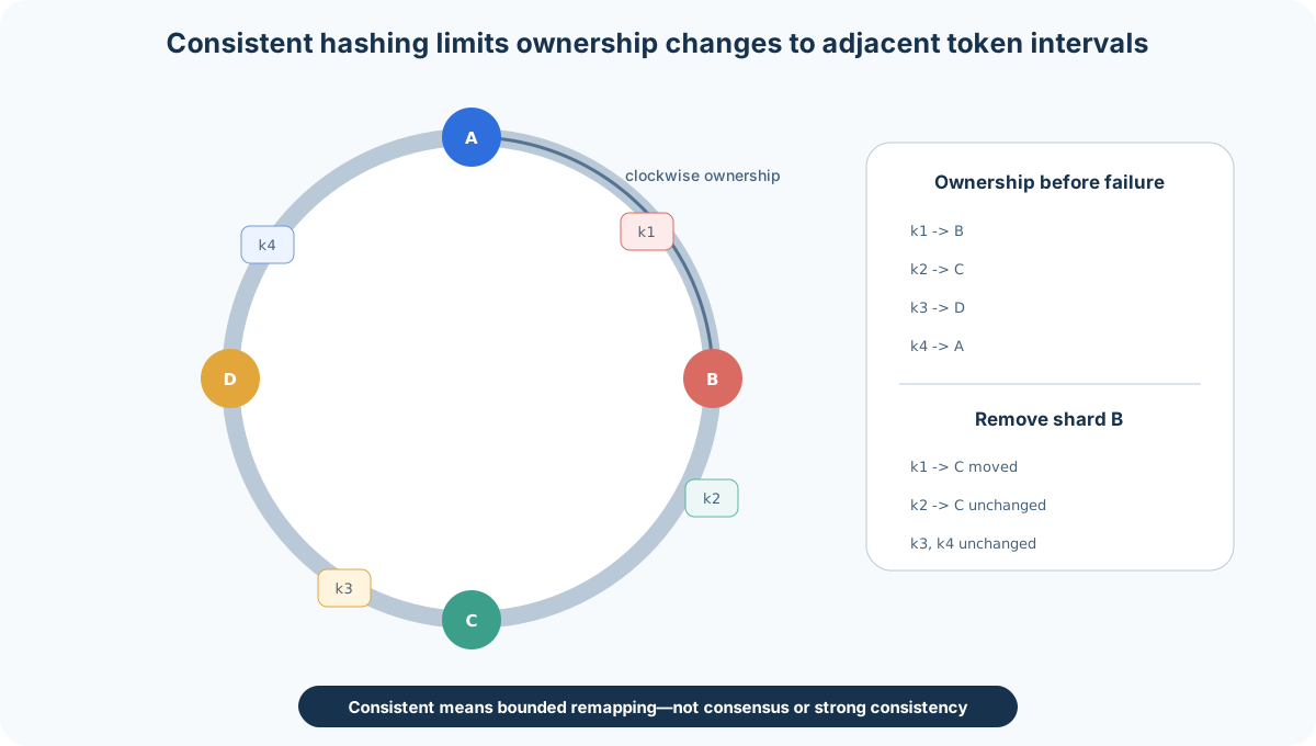
If shard B owns the token interval:
(token_A, token_B]
and B disappears, that interval moves to the next clockwise owner. Tokens owned by unrelated shards do not change.
Ring Lookup
Store sorted tokens and find the first token greater than or equal to the key hash:
from bisect import bisect_left


def ring_owner(key_hash, sorted_tokens, token_owners):
    index = bisect_left(sorted_tokens, key_hash)

    if index == len(sorted_tokens):
        index = 0

    return token_owners[sorted_tokens[index]]
Lookup is O(log t) for t tokens.
Bounded Disruption
When one equally sized owner out of n leaves, the ideal moved fraction is approximately:
1 / n
Only the departing owner’s keys need a new owner. Adding an owner similarly takes portions from existing intervals instead of recalculating every key.
“Consistent” refers to limited remapping under membership change. It does not mean strong consistency, consensus, or identical cluster views at every instant.
One Token Per Node Is Not Enough
Randomly placing one token per node creates uneven interval sizes. One node may own a much larger arc than another.
That motivates virtual nodes.
9. Virtual Nodes
Many Tokens Per Physical Node
A virtual node, or vnode, is one logical token assignment. Each physical node owns many vnodes spread around the ring:
node A -> tokens A1, A2, A3, ...
node B -> tokens B1, B2, B3, ...
node C -> tokens C1, C2, C3, ...
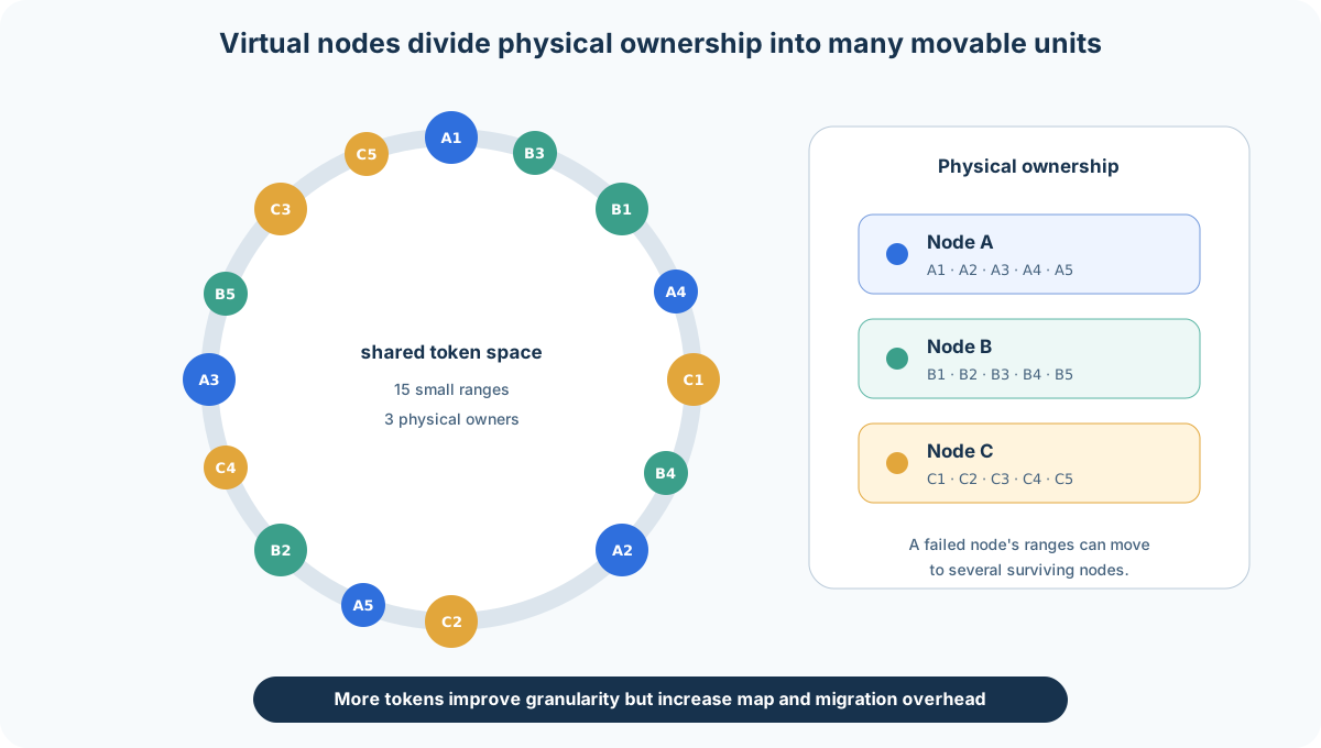
The benefits are:
- interval-size variance is averaged across many tokens;
- a failed node’s ranges are distributed among several survivors;
- heterogeneous machines can own different token counts;
- rebalancing can move small units rather than one large range.
The Cost of More Tokens
More virtual nodes create:
- larger routing maps;
- more replica-placement entries;
- more small files or per-range metadata in some engines;
- more migration tasks;
- more control-plane work.
The vnode count is therefore a granularity tradeoff, not a value to maximize.
Failure-Domain-Aware Replicas
Walking clockwise to choose the next (r-1) tokens is insufficient if several tokens belong to the same machine or rack. Replica placement must skip duplicate physical owners and satisfy topology rules:
primary vnode -> node A, zone 1
replica 2     -> node D, zone 2
replica 3     -> node G, zone 3
Logical distribution and physical failure domains must be modelled together.
10. Rendezvous Hashing
Highest-Score Ownership
Rendezvous, or highest-random-weight, hashing computes a score for every candidate owner:
score(key, shard) = hash(key, stable_shard_id)

owner(key) =
    shard with the highest score
def rendezvous_owner(key, shard_ids, stable_hash):
    return max(
        shard_ids,
        key=lambda shard_id: stable_hash(key, shard_id),
    )
When a shard is removed, only keys for which that shard had the highest score need a new owner. For every other key, the highest surviving score remains the same.
Ring Versus Rendezvous
Rendezvous hashing does not require an ordered ring or successor lookup. Its basic form scores every candidate, making lookup O(n) in the number of shards. Hierarchical or optimized forms reduce that cost.
Consistent-hash rings provide natural token intervals and vnode movement. Rendezvous hashing provides a compact selection rule and straightforward bounded disruption. Either can support weights, but weighted variants must be designed carefully; multiplying a raw score by weight is not generally a correct universal formulation.
Placement Is Not Migration
Both algorithms compute a desired owner. Neither transfers bytes, orders a cutover, repairs stale clients, or verifies that the target has caught up.
That distinction is fundamental:
placement algorithm -> where data should belong
migration protocol  -> how live ownership safely changes
11. Fixed Slots and Directory-Based Placement
Insert a Logical Namespace
A system does not need to hash keys directly onto nodes. It can introduce stable logical partitions:
key -> slot -> shard -> replica set
For example:
slot = hash(key) mod 4096

slots 0-1023    -> shard S1
slots 1024-2047 -> shard S2
slots 2048-3071 -> shard S3
slots 3072-4095 -> shard S4
Adding a shard does not change hash(key) mod 4096. The control plane moves selected slots to the new shard.
This is the model used by systems such as Redis Cluster, whose fixed slot namespace separates key hashing from physical ownership.
Why Indirection Helps
A stable partition ID provides:
- compact routing metadata;
- explicit movement units;
- versioned ownership;
- placement independent of node addresses;
- operational control over which ranges move;
- the ability to balance storage and traffic rather than token count alone.
The cost is a metadata map that must be stored, distributed, and refreshed.
Directory-Based Routing
The most flexible model records each partition in a directory:
| Partition | Key interval or rule | Replica group | Epoch | State |
|---|---|---|---|---|
| P17 | tenant 0-999 | G4 | 81 | serving |
| P18 | tenant 1000-1499 | G7 | 83 | migrating |
| P19 | tenant 1500-1999 | G2 | 79 | serving |
The directory can represent irregular ranges, tenant-specific placement, splits, merges, and explicit failure-domain rules.
The directory becomes critical control-plane state. It usually needs durable replication and ordered updates, often through a consensus-backed metadata service.
Routing Metadata Must Stay Small Enough
One routing entry per application row would recreate a distributed index in the routing layer. The logical partition count should be much larger than the node count for flexibility, but much smaller than the record count.
This yields a hierarchy:
billions of rows
-> thousands or millions of logical partitions
-> tens or hundreds of nodes
12. Metadata Versions and Stale Routers
Why an Epoch Is Required
Suppose partition P17 moves from shard A to shard B:
map version 81: P17 -> A
map version 82: P17 -> B
A client with version 81 may continue sending writes to A after the cutover. If A accepts them while B independently accepts version-82 writes, the system has two primaries.
Every ownership change therefore needs a monotonic version, generation, term, or fencing token.
Request and Owner Validation
A simplified request can carry:
partition = P17
observed_epoch = 81
operation = PUT k v
The receiver compares that epoch with its current ownership state:
RouteResult handle(const ShardRequest& request) {
    Ownership current = ownershipTable.lookup(request.partition);

    if (!current.is_local_primary) {
        return Redirect{
            .owner = current.primary,
            .epoch = current.epoch
        };
    }

    if (request.observed_epoch < current.epoch) {
        return RefreshRequired{.epoch = current.epoch};
    }

    return executeLocally(request);
}
The exact protocol differs by system, but the rule is stable: ownership claims must be validated against a version that orders topology changes.
Redirect, Forward, or Reject
A stale destination can:
- redirect the client to the current owner;
- forward the operation during a bounded transition;
- reject it and require metadata refresh.
Redirects keep the old node from remaining in the path. Forwarding can smooth client transitions but risks hiding permanently stale routers and adds another hop. Rejection is simple but makes topology change more visible to clients.
Metadata Propagation Is Eventually Consistent
Not every router learns version 82 simultaneously:
router R1 -> version 82
router R2 -> version 81
router R3 -> version 82
Temporary disagreement is acceptable only if storage owners enforce the ordered cutover. Client metadata convergence alone must not be the safety mechanism.
13. Hot Partitions and Skew
Three Different Kinds of Skew
Data skew means one shard stores more bytes.
Traffic skew means one shard receives more operations.
Cost skew means operations on one shard consume more CPU, I/O, or latency despite similar request counts.
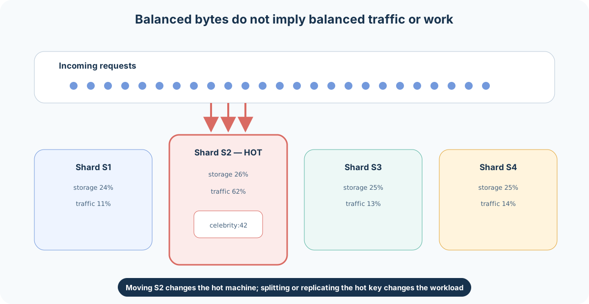
Moving a large cold partition may improve byte balance while making traffic balance worse.
Hot Keys
One key can dominate demand:
feature flag read by every server
celebrity profile
flash-sale inventory item
dominant tenant
global counter
No deterministic one-owner hash function can spread one key across owners without changing the data model or operation semantics.
Read-Hot Mitigations
Read-heavy immutable or slowly changing keys can use:
- replicas serving reads;
- application or edge caches;
- request coalescing;
- replicated materialized views;
- short-lived local copies with version validation.
The consistency requirement determines how stale those copies may be.
Write-Hot Mitigations
Writes require application-aware decomposition. A counter might be striped:
logical counter X
  -> X:0
  -> X:1
  -> X:2
  -> X:3
Writers choose a stripe. Readers aggregate them. This improves write parallelism but makes reads and atomic updates more expensive.
Time-series writes can add buckets:
(device_id, day, bucket)
Again, queries must fan out across buckets.
Hot Tenants
A multi-tenant shard key based only on tenant ID provides excellent isolation until one tenant exceeds a shard’s capacity.
Useful designs include:
- tenant-specific subshards;
- dedicated shards for dominant tenants;
- a directory mapping one tenant to several partitions;
- per-tenant admission control;
- workload-aware rebalancing.
This is why explicit directory or slot maps often outlive pure hash-to-node placement in mature systems.
14. Replication Inside Each Shard
Shard First, Then Replicate
For three logical shards and replication factor three:
S1 -> A1 primary, A2 replica, A3 replica
S2 -> B1 primary, B2 replica, B3 replica
S3 -> C1 primary, C2 replica, C3 replica
Each shard has its own replication protocol, log position, health, and failover state.
Sharding increases aggregate capacity because different shards can process independent operations in parallel. Replication improves availability and read capacity but consumes storage and write bandwidth.
Failure Domains
Replicas for one shard should not share the failure domain they protect against:
primary  -> zone A
replica  -> zone B
replica  -> zone C
Balancing primary ownership alone is insufficient. A placement plan must also balance replica count, replica traffic, disk usage, and recovery load across nodes and zones.
Promotion Does Not Change the Partition Function
If S2’s primary fails and a replica is promoted:
key -> logical shard S2
does not change. Only:
S2 -> current primary
changes.
This is another advantage of logical indirection: replica failover does not require rehashing application keys.
Avoid Immediate Permanent Rebalancing
A transient node outage should not automatically cause the entire lost replica set to be rebuilt and redistributed at maximum speed. If the node returns quickly, the movement was unnecessary and may have overloaded healthy nodes.
Systems commonly separate:
fast traffic failover
delayed permanent repair or rebalancing
The delay is a tradeoff between reduced redundancy and unnecessary movement.
15. Live Rebalancing
Desired Placement Is Not Current Ownership
Suppose P17 should move from source A to target B. The target cannot become authoritative merely because the control plane chose it. B first needs a consistent copy and must catch up with writes arriving during the copy.
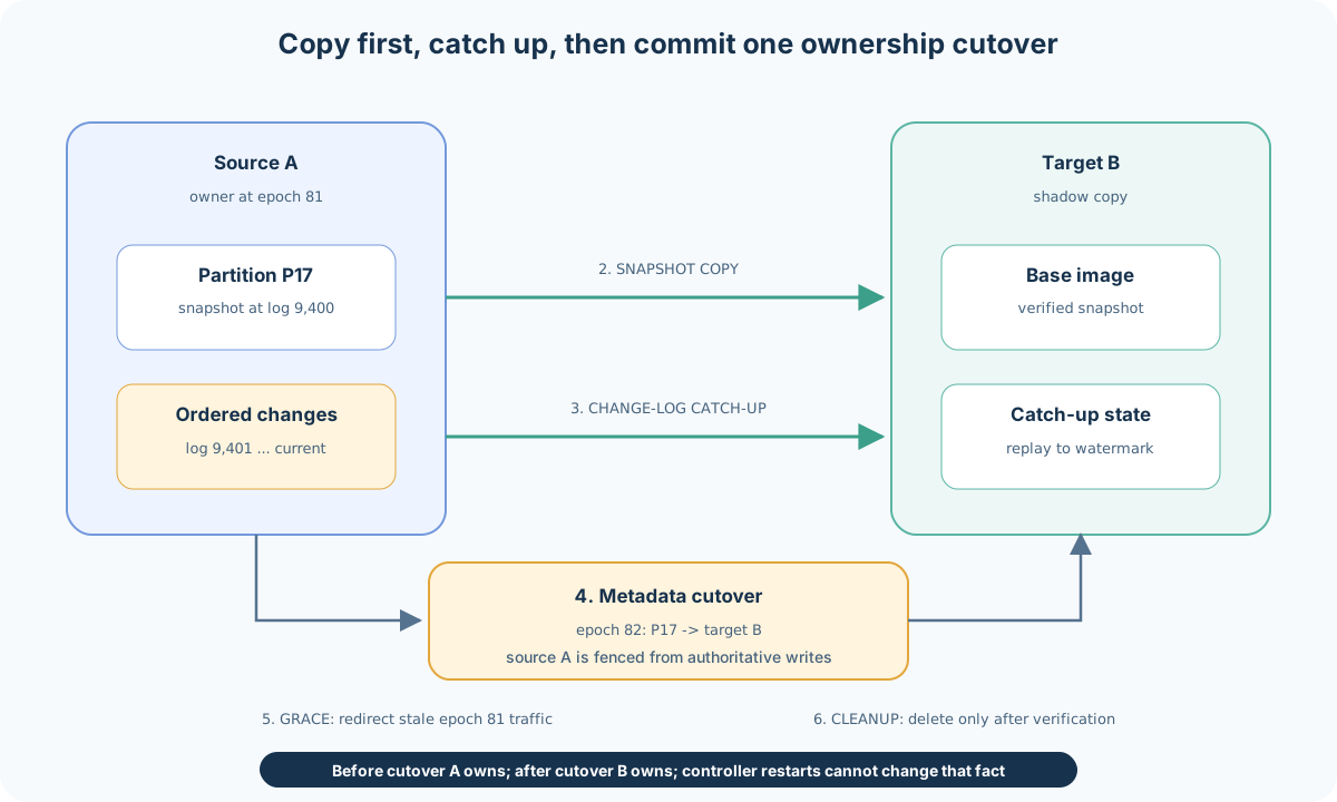
A Safe Migration Shape
A common sequence is:
1. PREPARE
   reserve capacity and record migration intent

2. SNAPSHOT
   copy a consistent base image from source to target

3. CATCH UP
   replay ordered changes after the snapshot position

4. CUT OVER
   commit metadata epoch e+1 with target as owner

5. GRACE
   source redirects or temporarily forwards stale traffic

6. CLEAN UP
   remove source data after safety checks and retention delay
The exact implementation may use a write-ahead log, change stream, Raft log, LSM file transfer, or storage snapshots.
Why Naive Dual Writes Are Dangerous
A router writing independently to A and B can observe:
write succeeds on A
write fails on B
router crashes before repair
Now copies diverge. A safer model keeps one authoritative write order during copy. The source records accepted changes, and the target replays that ordered stream until it reaches the cutover watermark.
Dual writes can be made correct with transaction or reconciliation machinery, but the phrase “write to both” is not itself a protocol.
The Cutover Point
At cutover:
epoch e:   source A may accept authoritative writes
epoch e+1: target B may accept authoritative writes
The control plane must serialize this transition. Source A must learn that its epoch is fenced before it can accept writes that conflict with B.
Some systems briefly pause writes, acquire a partition lease, or route all writes through a coordinator during the final boundary. The pause can be short if B is already caught up.
Migration Must Be Restartable
Every stage needs durable progress:
snapshot identifier
last copied key or file
change-log position
checksum state
committed ownership epoch
cleanup eligibility
If the process crashes, an operator or controller should determine whether to resume, roll back before cutover, or finish cleanup after cutover.
Invariant: cleanup must never delete the last authoritative copy.
16. Split, Merge, and Move
Moving Changes Placement
A move preserves the logical partition:
P17 on node A -> P17 on node B
Keys retain their partition ID. Only physical placement changes.
Splitting Changes Partition Boundaries
An oversized range:
P17 = [1000, 2000)
can split into:
P17 = [1000, 1500)
P42 = [1500, 2000)
The metadata operation must make the boundary atomic from the router’s perspective. A versioned map should not expose a gap or overlapping writable primaries.
Merging Reduces Fragmentation
Adjacent small partitions:
P17 = [1000, 1250)
P42 = [1250, 1500)
may merge after data ages or tenants shrink. Merging reduces per-partition metadata and small-file overhead, but it is live topology change and needs the same versioning discipline as a split.
Split Before a Partition Becomes Unmovable
Migration time is roughly:
copy time =
    bytes to move / effective migration bandwidth
A 2 TB shard copied at an effective 100 MB/s needs:
2,000,000 MB / 100 MB/s
    = 20,000 seconds
    = 5.6 hours
That excludes retries, verification, foreground contention, and catch-up. Smaller logical partitions create faster, safer recovery and rebalancing.
The tradeoff is more metadata and more units for the control plane to manage.
17. Cross-Shard Operations
Scatter and Gather
A query that does not contain the partition key may need every shard:
router sends query to S1, S2, S3, ... Sn
-> each shard computes local result
-> router merges results
Latency is influenced by the slowest participating shard. Total work grows with fanout. One overloaded shard can degrade the global query.
For top-K:
each shard returns local top K
coordinator merges n * K candidates
Pagination, ordering, failures, and concurrent writes make the merge more complex than concatenation.
Secondary Indexes
A local secondary index is partitioned with the base data. It efficiently answers predicates within a known partition key.
A global secondary index creates a second sharded dataset:
email -> user_id
Its partitioning may differ from the primary table. Updating both introduces transactional or eventual-consistency questions.
Cross-Shard Transactions
Single-shard transactions can use one shard’s local transaction and replication mechanism. A transaction touching multiple shards needs distributed coordination, commonly two-phase commit or an application-level alternative.
Sharding therefore changes transaction cost:
one shard -> local lock/log/commit path
many shards -> distributed prepare, commit, and recovery
Choosing a partition key that co-locates transactional data can remove an entire distributed protocol from the common path.
Unique Constraints
A uniqueness constraint is local only when the unique value determines the shard. Global username uniqueness, for example, may require:
- a separately sharded uniqueness index;
- a centralized allocator;
- a transaction across index and primary data;
- deterministic ownership based on username.
Schema guarantees must be designed together with partitioning.
18. Failure Semantics
Router Has Stale Metadata
The old owner redirects, forwards, or rejects using the newer epoch. The client refreshes its map and retries only when operation semantics permit.
For writes, an absent response is ambiguous: the old or new owner may have committed the operation before the response was lost. Idempotency keys or transaction identifiers may be required.
Source Fails During Copy
If a source replica fails before cutover, another replica may continue serving and producing the change stream. If the shard had no surviving authoritative copy, rebalancing cannot manufacture the missing data.
Migration planning must account for current replica health before intentionally removing another copy.
Target Fails Before Cutover
The source is still authoritative. The controller can discard target state and retry elsewhere. This is why ownership should not change at the beginning of a copy.
Controller Fails
Migration intent and progress must be durable. A replacement controller reads the state and decides:
before committed cutover -> source remains owner
after committed cutover  -> target remains owner
There must not be a state in which controller memory is the only evidence of the authoritative owner.
Network Partition Separates Source and Target
The metadata authority and fencing rule determine who may accept writes. If both sides independently decide they are primary, later byte comparison cannot always reconstruct the intended order.
This is why partition ownership is a consensus or lease problem even when key placement is based on hashing.
19. A Placement Simulator
Compare Movement and Distribution
The following Python program compares modulo, consistent-ring, and rendezvous placement using the same stable 64-bit hash:
from bisect import bisect_left
from collections import Counter
from hashlib import blake2b


def hash64(value: str) -> int:
    digest = blake2b(
        value.encode("utf-8"),
        digest_size=8,
    ).digest()
    return int.from_bytes(digest, "big")


def modulo_owner(key: str, nodes: list[str]) -> str:
    return nodes[hash64(key) % len(nodes)]


class ConsistentHashRing:
    def __init__(
        self,
        nodes: list[str],
        virtual_nodes: int = 200,
    ):
        token_owner: dict[int, str] = {}

        for node in nodes:
            for vnode in range(virtual_nodes):
                token = hash64(f"{node}#{vnode}")
                if token in token_owner:
                    raise RuntimeError("token collision")
                token_owner[token] = node

        self.tokens = sorted(token_owner)
        self.token_owner = token_owner

    def owner(self, key: str) -> str:
        token = hash64(key)
        index = bisect_left(self.tokens, token)

        if index == len(self.tokens):
            index = 0

        return self.token_owner[self.tokens[index]]


def rendezvous_owner(
    key: str,
    nodes: list[str],
) -> str:
    return max(
        nodes,
        key=lambda node: hash64(f"{key}|{node}"),
    )


def movement_fraction(before, after, keys) -> float:
    moved = sum(
        before(key) != after(key)
        for key in keys
    )
    return moved / len(keys)


def distribution(owner, keys) -> Counter:
    return Counter(owner(key) for key in keys)


def skew(counts: Counter) -> float:
    average = sum(counts.values()) / len(counts)
    return max(counts.values()) / average


keys = [f"key-{index}" for index in range(100_000)]
before_nodes = ["A", "B", "C", "D"]
after_nodes = ["A", "B", "C", "D", "E"]

ring_before = ConsistentHashRing(before_nodes)
ring_after = ConsistentHashRing(after_nodes)

strategies = {
    "modulo": (
        lambda key: modulo_owner(key, before_nodes),
        lambda key: modulo_owner(key, after_nodes),
    ),
    "ring-200-vnodes": (
        ring_before.owner,
        ring_after.owner,
    ),
    "rendezvous": (
        lambda key: rendezvous_owner(key, before_nodes),
        lambda key: rendezvous_owner(key, after_nodes),
    ),
}

for name, (before, after) in strategies.items():
    moved = movement_fraction(before, after, keys)
    after_counts = distribution(after, keys)

    print(
        f"{name:18s} "
        f"moved={moved:6.2%} "
        f"skew={skew(after_counts):.3f}"
    )
One deterministic run produces:
modulo             moved=80.10% skew=1.010
ring-200-vnodes    moved=20.16% skew=1.069
rendezvous         moved=19.91% skew=1.008
The precise results depend on the hash, keys, and vnode count. The structural result is more important:
- modulo hashing balances the final key count but remaps most keys;
- a vnode ring limits movement with some finite-sample interval skew;
- rendezvous hashing limits movement and distributes this sample evenly.
The simulator models desired ownership only. It does not implement replication, metadata epochs, or byte transfer.
20. End-to-End Rebalancing Example
Initial State
Consider an event store using:
partition key = tenant_id
clustering key = event_time
The map at epoch 80 is:
P17: tenants [0, 1000)    -> shard A
P18: tenants [1000, 2000) -> shard B
P19: tenants [2000, 3000) -> shard C
Each shard has three replicas across three zones.
Detecting the Problem
Shard B stores 30 percent of bytes but serves 65 percent of writes because tenant 1450 has grown rapidly.
Moving all of P18 to another node changes which machine is hot but does not split the workload. The control plane chooses a boundary change:
P18: tenants [1000, 1450)
P42: tenant 1450 with 16 write buckets
P43: tenants (1450, 2000)
This is an application-aware split. The hot tenant receives independent subpartitions; neighboring tenants remain range partitioned.
Copy and Catch-Up
- The metadata service records migration intent at epoch 81.
- Target replica groups reserve disk and network capacity.
- Source B takes a snapshot at log position 9,400.
- Targets copy the relevant base ranges.
- Source B continues accepting writes and retains changes after position 9,400.
- Targets replay the change stream.
- Checksums and record counts verify the copied state.
- Targets reach the current log watermark.
During these stages, B remains authoritative.
Cutover
The metadata service commits epoch 82:
P18 -> target group D
P42 -> target group E
P43 -> target group F
New routers use epoch 82. Source B rejects authoritative epoch-82 writes and redirects stale epoch-81 traffic.
After the grace period, metrics show no stale traffic and the controller marks the old ranges eligible for deletion.
Failure During Cleanup
If the cleanup worker crashes after deleting only one old range, ownership does not change: epoch 82 already names D, E, and F. Cleanup resumes idempotently from durable progress.
The operation is safe because copying, ownership cutover, and deletion are separate stages with a single committed cutover point.
21. Operating Shards at Scale
Monitor the Unit That Moves
Per-node averages can hide one bad partition. Collect per-partition:
- stored bytes;
- row or object count;
- read and write rate;
- CPU and storage time;
- p50, p95, and p99 latency;
- replica lag;
- compaction and repair work;
- cache hit ratio;
- tenant concentration.
The metrics need stable partition IDs so behavior can be followed across node movement.
Choose a Maximum Useful Partition Size
A maximum is constrained by:
- recovery time objective;
- migration bandwidth;
- snapshot and backup duration;
- compaction behavior;
- per-partition metadata overhead;
- hotspot isolation granularity.
If a partition cannot move or rebuild within the recovery objective, it is too large even if it fits on one disk.
Rate-Limit Rebalancing
Migration competes with foreground traffic for:
source reads
target writes
network bandwidth
CPU
compaction capacity
replication bandwidth
Controllers should enforce per-node and global movement budgets, prioritize restoring lost redundancy, and pause lower-priority balancing when user latency degrades.
Leave Failure Headroom
If every node is 90 percent full, losing one node may leave nowhere to place its replicas. Storage capacity planning must include:
- one node or zone unavailable;
- temporary source and target copies during movement;
- compaction headroom;
- uneven partition sizes;
- growth during a migration.
Test the Control Path
Failure drills should include:
- stale router after a cutover;
- source crash during snapshot;
- target crash during catch-up;
- controller restart at every migration stage;
- metadata-service partition;
- checksum mismatch;
- cleanup retry;
- concurrent split and replica failure.
The cluster’s ability to serve traffic today does not prove it can change ownership safely tomorrow.
22. Choosing a Strategy
Comparison
| Strategy | Locality | Balance | Movement under change | Metadata | Best fit |
|---|---|---|---|---|---|
| Range partitioning | Strong ordered locality | Sensitive to key distribution | Explicit ranges move | Boundaries | Range scans, tablets |
| Modulo hashing | None beyond exact key | Good with uniform hashes | Most keys remap | Minimal | Fixed ephemeral pools |
| Consistent ring | Hash locality only | Improved with vnodes | Bounded | Token ring | Caches, Dynamo-style systems |
| Rendezvous hashing | Hash locality only | Good | Bounded | Stable node list | Client or proxy selection |
| Fixed slots | Hash locality only | Operator controlled | Selected slots move | Slot map | Explicit online rebalancing |
| Directory | Arbitrary | Workload aware | Explicit partitions move | Largest and critical | Mature databases, tenant placement |
Decision Questions
Choose by answering:
Do dominant queries require ordered ranges?
Can the partition key be present in every common request?
Can one tenant or key exceed a shard's capacity?
How often does membership change?
What is the maximum acceptable movement?
Who stores and distributes the partition map?
How are stale owners fenced?
How long may a partition take to move or rebuild?
Which operations require cross-shard transactions?
Which failure domain must replicas survive?
The choice is rarely “range or hash” in isolation. Production systems often combine:
directory-managed logical partitions
-> hash-distributed by partition key
-> ordered by clustering key within a partition
-> replicated across failure domains
23. Conclusion
Sharding is the mechanism that turns one storage node’s keyspace into many independently owned units. Its steady-state path is simple:
application key
  -> partition key
  -> logical partition
  -> current replica group
  -> local storage operation
The hard part is change.
Range partitioning preserves order but can concentrate a moving write frontier. Hash partitioning spreads keys but destroys global range locality. Consistent and rendezvous hashing limit remapping under membership change. Virtual nodes smooth interval variance. Fixed slots and directories add explicit control over movement and workload-aware placement.
None of those algorithms is a live migration protocol. Safe rebalancing keeps one authoritative write order while a target copies and catches up, commits one versioned ownership cutover, fences stale owners, preserves a grace period for routers, and deletes source data only after verification.
The most important operational lesson is that balanced key count is not balanced work. Hot keys, dominant tenants, range frontiers, replica recovery, and cross-shard fanout all require measurement at the partition level. Partitions should remain small enough to split, move, rebuild, and verify within the system’s recovery objective.
A successful sharding design therefore combines three disciplines:
placement policy
+ versioned ownership protocol
+ workload-aware operations
Hashing answers where data should go. The rest of the system makes that answer safe while the cluster changes.
Leave a Comment